The same plot in 14 other libraries — Python: Altair, Bokeh, lets-plot, Matplotlib, Plotly, plotnine, Pygal, Seaborn; R: ggplot2; JavaScript: Chart.js, D3.js, Apache ECharts, Highcharts, MUI X Charts. Compare all 15 side by side: Beer-Lambert Calibration Curve in Python, R, Julia and JavaScript.
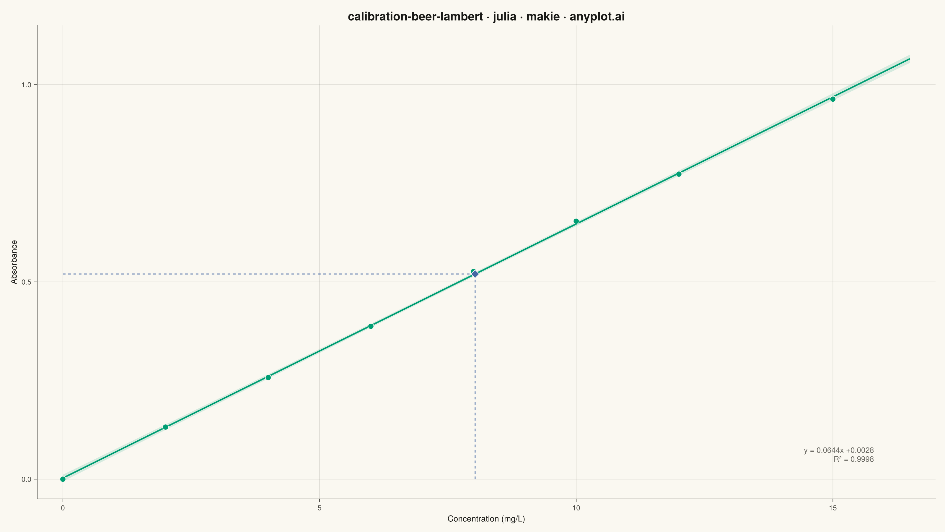
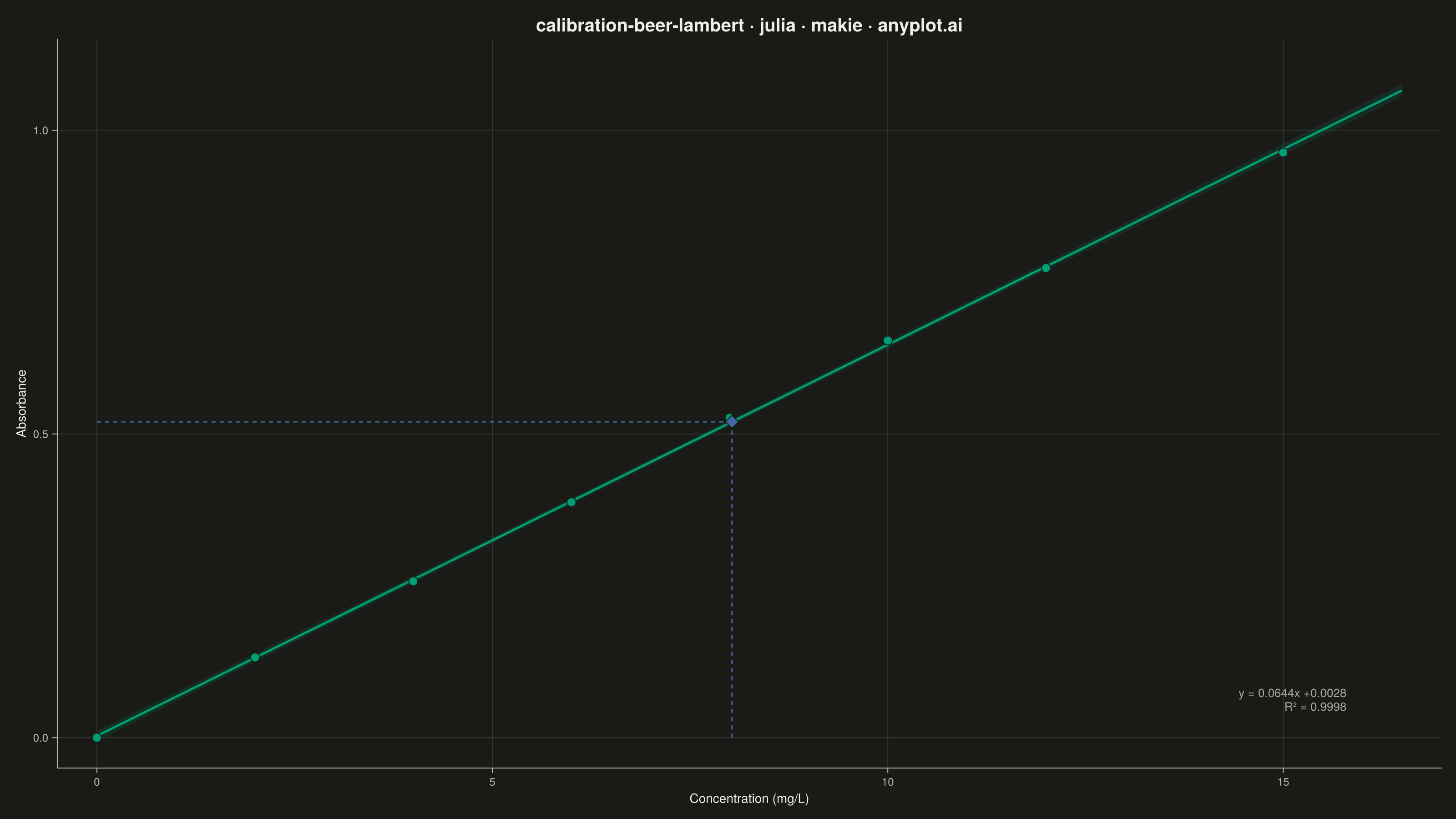
A calibration curve plotting absorbance versus concentration following Beer-Lambert law (A = εlc). Measured calibration standards are shown as scatter points with a linear regression fit line. The regression equation (y = mx + b) and R² value are displayed on the plot. An example unknown sample is marked with dashed lines extending to both axes, demonstrating how the curve is used to determine concentration from a measured absorbance. This plot is fundamental in analytical chemistry for quantitative spectrophotometric analysis.
# anyplot.ai
# calibration-beer-lambert: Beer-Lambert Calibration Curve
# Library: makie 0.22.10 | Julia 1.11.9
# Quality: 91/100 | Created: 2026-06-03

using CairoMakie
using Colors
using Random
using Statistics
using Printf

Random.seed!(42)

# Theme tokens (Imprint palette — theme-adaptive chrome)
const THEME       = get(ENV, "ANYPLOT_THEME", "light")
const PAGE_BG     = THEME == "light" ? colorant"#FAF8F1" : colorant"#1A1A17"
const ELEVATED_BG = THEME == "light" ? colorant"#FFFDF6" : colorant"#242420"
const INK         = THEME == "light" ? colorant"#1A1A17" : colorant"#F0EFE8"
const INK_SOFT    = THEME == "light" ? colorant"#4A4A44" : colorant"#B8B7B0"
const INK_MUTED   = THEME == "light" ? colorant"#6B6A63" : colorant"#A8A79F"

const IMPRINT_PALETTE = [
    colorant"#009E73",  # 1 — Imprint brand green (always first series)
    colorant"#C475FD",  # 2 — lavender
    colorant"#4467A3",  # 3 — blue
    colorant"#BD8233",  # 4 — ochre
    colorant"#AE3030",  # 5 — matte red
    colorant"#2ABCCD",  # 6 — cyan
    colorant"#954477",  # 7 — rose
    colorant"#99B314",  # 8 — lime
]

# Data — nitrate colorimetric assay, UV-Vis at 540 nm (environmental water testing)
concentrations = Float64[0.0, 2.0, 4.0, 6.0, 8.0, 10.0, 12.0, 15.0]  # mg/L
true_abs = 0.065 .* concentrations  # Beer-Lambert: A = εlc, εl ≈ 0.065 L/mg
noise = randn(length(concentrations)) .* 0.008
absorbance = true_abs .+ noise
absorbance[1] = max(0.0, absorbance[1])  # blank must be non-negative

# Linear regression (ordinary least squares)
n = length(concentrations)
x_mean = mean(concentrations)
y_mean = mean(absorbance)
sxx = sum((concentrations .- x_mean) .^ 2)
sxy = sum((concentrations .- x_mean) .* (absorbance .- y_mean))
slope = sxy / sxx
intercept = y_mean - slope * x_mean

# Goodness of fit
y_pred_cal = slope .* concentrations .+ intercept
ss_res = sum((absorbance .- y_pred_cal) .^ 2)
ss_tot = sum((absorbance .- y_mean) .^ 2)
r_squared = 1.0 - ss_res / ss_tot

# Regression line and 95% prediction interval
x_fit = collect(range(0.0, 16.5, length=300))
y_fit = slope .* x_fit .+ intercept
s2 = ss_res / (n - 2)  # mean squared error
se_pred = sqrt.(s2 .* (1.0 ./ n .+ (x_fit .- x_mean) .^ 2 ./ sxx))
t_crit = 2.447  # t(0.025, df=6) for 95% prediction interval
y_upper = y_fit .+ t_crit .* se_pred
y_lower = y_fit .- t_crit .* se_pred

# Unknown sample: determine concentration from measured absorbance
unknown_abs = 0.520
unknown_conc = (unknown_abs - intercept) / slope

# Annotation string
eq_str = @sprintf("y = %.4fx %+.4f\nR² = %.4f", slope, intercept, r_squared)

# Plot
fig = Figure(
    size            = (1600, 900),
    fontsize        = 14,
    backgroundcolor = PAGE_BG,
)

ax = Axis(
    fig[1, 1];
    title              = "calibration-beer-lambert · julia · makie · anyplot.ai",
    titlesize          = 20,
    titlecolor         = INK,
    xlabel             = "Concentration (mg/L)",
    ylabel             = "Absorbance",
    xlabelsize         = 14,
    ylabelsize         = 14,
    xticklabelsize     = 12,
    yticklabelsize     = 12,
    xlabelcolor        = INK,
    ylabelcolor        = INK,
    xticklabelcolor    = INK_SOFT,
    yticklabelcolor    = INK_SOFT,
    xtickcolor         = INK_SOFT,
    ytickcolor         = INK_SOFT,
    backgroundcolor    = PAGE_BG,
    topspinevisible    = false,
    rightspinevisible  = false,
    leftspinecolor     = INK_SOFT,
    bottomspinecolor   = INK_SOFT,
    xgridcolor         = RGBAf(INK.r, INK.g, INK.b, 0.12),
    ygridcolor         = RGBAf(INK.r, INK.g, INK.b, 0.12),
    xminorgridvisible  = false,
    yminorgridvisible  = false,
)

# 95% prediction interval band
band!(ax, x_fit, y_lower, y_upper;
    color = (IMPRINT_PALETTE[1], 0.15),
    label = "95% Prediction interval")

# Regression line
lines!(ax, x_fit, y_fit;
    color     = IMPRINT_PALETTE[1],
    linewidth = 2.5,
    label     = "Linear fit")

# Calibration standard points
scatter!(ax, concentrations, absorbance;
    color       = IMPRINT_PALETTE[1],
    markersize  = 14,
    strokecolor = PAGE_BG,
    strokewidth = 1,
    label       = "Calibration standards",
)

# Dashed guide lines for unknown sample determination (no legend entry)
lines!(ax, [0.0, unknown_conc], [unknown_abs, unknown_abs];
    color     = IMPRINT_PALETTE[3],
    linewidth = 1.5,
    linestyle = :dash,
)
lines!(ax, [unknown_conc, unknown_conc], [0.0, unknown_abs];
    color     = IMPRINT_PALETTE[3],
    linewidth = 1.5,
    linestyle = :dash,
)

# Unknown sample marker
scatter!(ax, [unknown_conc], [unknown_abs];
    color       = IMPRINT_PALETTE[3],
    markersize  = 16,
    marker      = :diamond,
    strokecolor = PAGE_BG,
    strokewidth = 1,
    label       = "Unknown sample (A = 0.520)",
)

# Regression equation and R² annotation (lower-right area, data coordinates)
text!(ax, 15.8, 0.04;
    text     = eq_str,
    align    = (:right, :bottom),
    color    = INK_MUTED,
    fontsize = 15,
)

xlims!(ax, -0.5, 17.0)
ylims!(ax, -0.05, 1.15)

# Legend — identifies all four visual elements for unfamiliar readers
axislegend(ax;
    position        = :lt,
    labelcolor      = INK,
    labelsize       = 12,
    framecolor      = INK_SOFT,
    backgroundcolor = ELEVATED_BG,
    framevisible    = true,
)

# Save
save("plot-$(THEME).png", fig; px_per_unit = 2)
Runnable source as JSON, for any HTTP client: https://api.anyplot.ai/specs/calibration-beer-lambert/makie/code. Any spec id and library id listed in llms-full.txt fit the same URL shape; every URL below is complete and callable.
{
  "spec_id": "calibration-beer-lambert",
  "language": "julia",
  "library": "makie",
  "page": "https://anyplot.ai/calibration-beer-lambert/julia/makie",
  "hub": "https://anyplot.ai/calibration-beer-lambert",
  "code_json": "https://api.anyplot.ai/specs/calibration-beer-lambert/makie/code",
  "spec_json": "https://api.anyplot.ai/specs/calibration-beer-lambert",
  "render_light_png": "https://storage.googleapis.com/anyplot-images/plots/calibration-beer-lambert/julia/makie/plot-light.png",
  "render_dark_png": "https://storage.googleapis.com/anyplot-images/plots/calibration-beer-lambert/julia/makie/plot-dark.png",
  "quality_score": 91.0,
  "license": "MIT",
  "guide": "https://anyplot.ai/llms.txt"
}
Part of Beer-Lambert Calibration Curve on anyplot.ai.