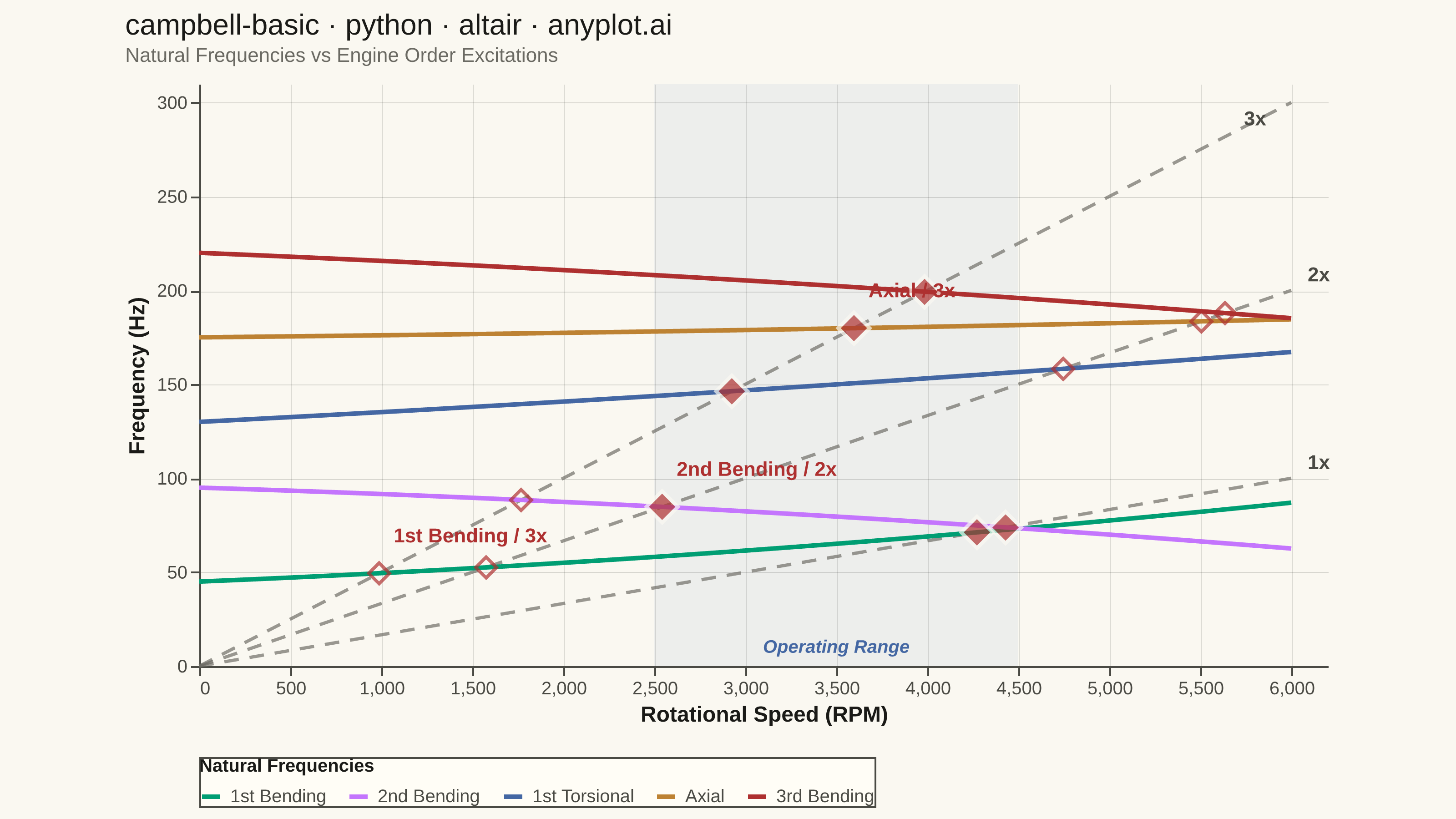
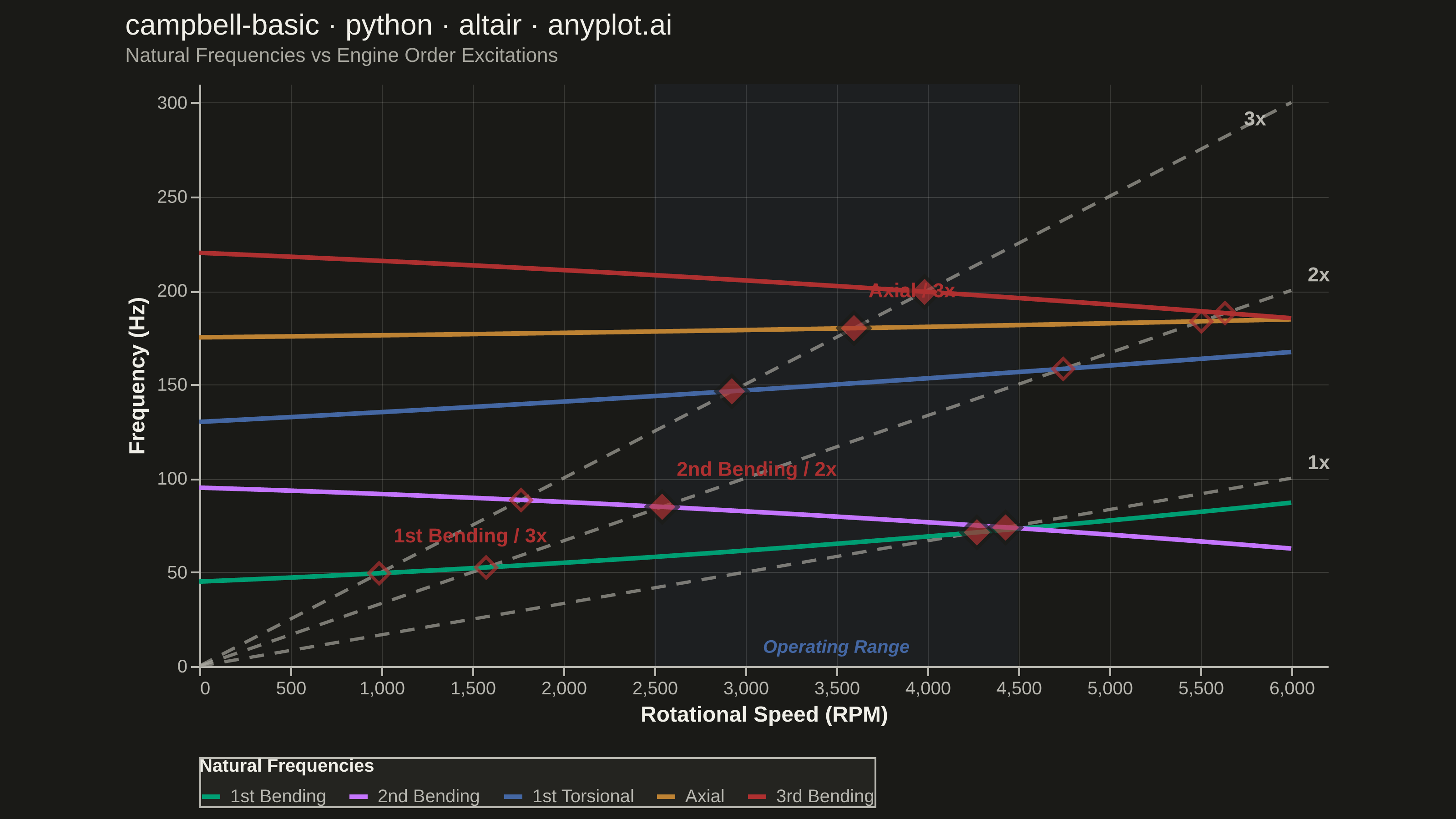
A Campbell Diagram (also called an interference diagram) plots natural frequencies against rotational speed to identify critical speeds and resonance conditions in rotating machinery. It overlays engine order excitation lines (diagonal lines from the origin) on top of natural frequency curves, with intersections marking critical speeds where resonance may occur. This visualization is essential for ensuring safe operating ranges in turbomachinery, automotive powertrains, and other rotating equipment.
""" anyplot.ai
campbell-basic: Campbell Diagram
Library: altair 6.1.0 | Python 3.13.13
Quality: 87/100 | Updated: 2026-05-28
"""

import sys


if sys.path and not sys.path[0].endswith("site-packages"):
    sys.path = [p for p in sys.path if "implementations/python" not in p]

import os

import altair as alt
import numpy as np
import pandas as pd
from PIL import Image


# Theme tokens
THEME = os.getenv("ANYPLOT_THEME", "light")
PAGE_BG = "#FAF8F1" if THEME == "light" else "#1A1A17"
ELEVATED_BG = "#FFFDF6" if THEME == "light" else "#242420"
INK = "#1A1A17" if THEME == "light" else "#F0EFE8"
INK_SOFT = "#4A4A44" if THEME == "light" else "#B8B7B0"
INK_MUTED = "#6B6A63" if THEME == "light" else "#A8A79F"
IMPRINT_PALETTE = ["#009E73", "#C475FD", "#4467A3", "#BD8233", "#AE3030", "#2ABCCD", "#954477", "#99B314"]

# Data — low-speed industrial machinery operating range 2500–4500 RPM
np.random.seed(42)
speeds = np.linspace(0, 6000, 80)

mode_labels = ["1st Bending", "2nd Bending", "1st Torsional", "Axial", "3rd Bending"]
base_freqs = [45, 95, 130, 175, 220]
slopes = [0.004, -0.003, 0.005, 0.001, -0.004]
curvatures = [5e-7, -4e-7, 2e-7, 1e-7, -3e-7]

mode_rows = []
for label, base, slope, curv in zip(mode_labels, base_freqs, slopes, curvatures, strict=True):
    freqs = base + slope * speeds + curv * speeds**2
    for s, f in zip(speeds, freqs, strict=True):
        mode_rows.append({"RPM": s, "Hz": f, "Mode": label})

engine_orders = [1, 2, 3]
eo_rows = []
for order in engine_orders:
    for s in speeds:
        eo_rows.append({"RPM": s, "Hz": order * s / 60, "EO": f"{order}x"})

df_modes = pd.DataFrame(mode_rows)
df_eo = pd.DataFrame(eo_rows)

# Dense sign-change detection for critical speed intersections
critical_rows = []
dense_speeds = np.linspace(0, 6000, 5000)
for label, base, slope, curv in zip(mode_labels, base_freqs, slopes, curvatures, strict=True):
    mode_freq = base + slope * dense_speeds + curv * dense_speeds**2
    for order in engine_orders:
        eo_freq = order * dense_speeds / 60
        diff = mode_freq - eo_freq
        sign_changes = np.where(np.diff(np.sign(diff)))[0]
        for idx in sign_changes:
            s_crit = dense_speeds[idx]
            f_crit = eo_freq[idx]
            if 100 < s_crit < 5900 and 5 < f_crit < 295:
                in_op = 2500 <= s_crit <= 4500
                critical_rows.append(
                    {"RPM": round(s_crit), "Hz": round(f_crit, 1), "Label": f"{label} / {order}x", "InOpRange": in_op}
                )

df_critical = pd.DataFrame(critical_rows)
df_crit_out = df_critical[~df_critical["InOpRange"]]
df_crit_in = df_critical[df_critical["InOpRange"]]

# Select 2–3 key annotations: one outside + up to two within operating range
key_out = df_crit_out.sort_values("Hz")
key_in = df_crit_in.sort_values("RPM")
annot_rows = []
if len(key_out) > 0:
    annot_rows.append(key_out.iloc[0].to_dict())
if len(key_in) > 0:
    annot_rows.append(key_in.iloc[0].to_dict())
if len(key_in) > 2:
    annot_rows.append(key_in.iloc[2].to_dict())
df_annot = pd.DataFrame(annot_rows) if annot_rows else pd.DataFrame(columns=df_critical.columns)

# Chart scales
op_min, op_max = 2500, 4500
x_scale = alt.Scale(domain=[0, 6200], nice=False)
y_scale = alt.Scale(domain=[0, 310])

# Operating range shaded band
op_band = (
    alt.Chart(pd.DataFrame({"x": [op_min], "x2": [op_max]}))
    .mark_rect(opacity=0.07, color=IMPRINT_PALETTE[2])
    .encode(x=alt.X("x:Q", scale=x_scale), x2="x2:Q")
)

# Operating range label
op_label = (
    alt.Chart(pd.DataFrame({"RPM": [(op_min + op_max) / 2], "Hz": [10], "label": ["Operating Range"]}))
    .mark_text(fontSize=10, fontStyle="italic", fontWeight="bold", color=IMPRINT_PALETTE[2])
    .encode(x=alt.X("RPM:Q", scale=x_scale), y=alt.Y("Hz:Q", scale=y_scale), text="label:N")
)

# Engine order excitation lines — dashed, muted, opacity raised from 0.55 to 0.68
eo_chart = (
    alt.Chart(df_eo)
    .mark_line(strokeWidth=1.8, strokeDash=[8, 6], opacity=0.68, color=INK_MUTED)
    .encode(x=alt.X("RPM:Q", scale=x_scale), y=alt.Y("Hz:Q", scale=y_scale), detail="EO:N")
)

# Engine order labels at right edge (direct labeling instead of legend)
eo_label_rows = []
for order in engine_orders:
    end_hz = order * 6000 / 60
    if end_hz <= 295:
        eo_label_rows.append({"RPM": 6050, "Hz": end_hz, "label": f"{order}x"})
    else:
        cap_rpm = 285 * 60 / order
        eo_label_rows.append({"RPM": cap_rpm, "Hz": 283, "label": f"{order}x"})

eo_labels = (
    alt.Chart(pd.DataFrame(eo_label_rows))
    .mark_text(fontSize=11, fontWeight="bold", align="left", dx=4, dy=-8, color=INK_SOFT)
    .encode(x=alt.X("RPM:Q", scale=x_scale), y=alt.Y("Hz:Q", scale=y_scale), text="label:N")
)

# Natural frequency mode curves
modes_chart = (
    alt.Chart(df_modes)
    .mark_line(strokeWidth=2.5)
    .encode(
        x=alt.X("RPM:Q", title="Rotational Speed (RPM)", scale=x_scale),
        y=alt.Y("Hz:Q", title="Frequency (Hz)", scale=y_scale),
        color=alt.Color(
            "Mode:N",
            scale=alt.Scale(domain=mode_labels, range=IMPRINT_PALETTE[:5]),
            legend=alt.Legend(
                title="Natural Frequencies", titleFontSize=10, labelFontSize=10, symbolStrokeWidth=2.5, symbolSize=100
            ),
        ),
    )
)

# Critical speed markers — outlined diamonds outside operating range
crit_out_chart = (
    alt.Chart(df_crit_out)
    .mark_point(size=130, shape="diamond", filled=False, strokeWidth=1.8)
    .encode(
        x=alt.X("RPM:Q", scale=x_scale),
        y=alt.Y("Hz:Q", scale=y_scale),
        color=alt.value(IMPRINT_PALETTE[4]),
        tooltip=["Label:N", "RPM:Q", "Hz:Q"],
    )
)

# Larger filled diamonds inside operating range — danger emphasis
crit_in_chart = (
    alt.Chart(df_crit_in)
    .mark_point(size=300, shape="diamond", filled=True, stroke=PAGE_BG, strokeWidth=2.0)
    .encode(
        x=alt.X("RPM:Q", scale=x_scale),
        y=alt.Y("Hz:Q", scale=y_scale),
        color=alt.value(IMPRINT_PALETTE[4]),
        tooltip=["Label:N", "RPM:Q", "Hz:Q"],
    )
)

# Consolidated annotation layer for key critical speeds (single layer, not per-row)
annot_chart = (
    alt.Chart(df_annot)
    .mark_text(fontSize=11, fontWeight="bold", align="left", dx=8, dy=-20)
    .encode(
        x=alt.X("RPM:Q", scale=x_scale),
        y=alt.Y("Hz:Q", scale=y_scale),
        text="Label:N",
        color=alt.value(IMPRINT_PALETTE[4]),
    )
)

# Compose layers
layers = [op_band, eo_chart, modes_chart, crit_out_chart, crit_in_chart, eo_labels, op_label]
if len(df_annot) > 0:
    layers.append(annot_chart)

combined = layers[0]
for lyr in layers[1:]:
    combined = combined + lyr

title_str = "campbell-basic · python · altair · anyplot.ai"

chart = (
    combined.properties(
        width=620,
        height=320,
        background=PAGE_BG,
        padding={"left": 0, "right": 0, "top": 0, "bottom": 0},
        title=alt.Title(
            title_str,
            fontSize=16,
            fontWeight=500,
            anchor="start",
            color=INK,
            subtitle="Natural Frequencies vs Engine Order Excitations",
            subtitleFontSize=11,
            subtitleColor=INK_MUTED,
        ),
    )
    .configure_view(fill=PAGE_BG, stroke=None)
    .configure_axis(
        domainColor=INK_SOFT,
        tickColor=INK_SOFT,
        gridColor=INK,
        gridOpacity=0.15,
        gridWidth=0.5,
        labelColor=INK_SOFT,
        labelFontSize=10,
        titleColor=INK,
        titleFontSize=12,
        tickSize=5,
    )
    .configure_legend(
        fillColor=ELEVATED_BG,
        strokeColor=INK_SOFT,
        labelColor=INK_SOFT,
        labelFontSize=10,
        titleColor=INK,
        titleFontSize=10,
        symbolStrokeWidth=2.5,
        symbolSize=100,
        orient="bottom",
        columns=5,
    )
    .configure_title(anchor="start", offset=10, color=INK)
)

# Save — canvas gate: inner view 620×320 @ scale 4.0 → target 3200×1800 with padding
TW, TH = 3200, 1800
chart.save(f"plot-{THEME}.png", scale_factor=4.0)

_img = Image.open(f"plot-{THEME}.png").convert("RGB")
_w, _h = _img.size
if _w > TW or _h > TH:
    raise SystemExit(
        f"altair vl-convert produced {_w}×{_h}, exceeds target {TW}×{TH}. "
        f"Shrink chart .properties(width=, height=) values and re-render."
    )
if _w < TW or _h < TH:
    _canvas = Image.new("RGB", (TW, TH), PAGE_BG)
    _canvas.paste(_img, ((TW - _w) // 2, (TH - _h) // 2))
    _canvas.save(f"plot-{THEME}.png")

chart.save(f"plot-{THEME}.html")
Runnable source as JSON, for any HTTP client: https://api.anyplot.ai/specs/campbell-basic/altair/code. Any spec id and library id listed in llms-full.txt fit the same URL shape; every URL below is complete and callable.
{
  "spec_id": "campbell-basic",
  "language": "python",
  "library": "altair",
  "page": "https://anyplot.ai/campbell-basic/python/altair",
  "hub": "https://anyplot.ai/campbell-basic",
  "code_json": "https://api.anyplot.ai/specs/campbell-basic/altair/code",
  "spec_json": "https://api.anyplot.ai/specs/campbell-basic",
  "render_light_png": "https://storage.googleapis.com/anyplot-images/plots/campbell-basic/python/altair/plot-light.png",
  "render_dark_png": "https://storage.googleapis.com/anyplot-images/plots/campbell-basic/python/altair/plot-dark.png",
  "interactive_light_html": "https://storage.googleapis.com/anyplot-images/plots/campbell-basic/python/altair/plot-light.html",
  "interactive_dark_html": "https://storage.googleapis.com/anyplot-images/plots/campbell-basic/python/altair/plot-dark.html",
  "quality_score": 87.0,
  "license": "MIT",
  "guide": "https://anyplot.ai/llms.txt"
}
Part of Campbell Diagram on anyplot.ai.