The same plot in 14 other libraries — Python: Altair, Bokeh, lets-plot, Matplotlib, Plotly, plotnine, Pygal, Seaborn; Julia: Makie.jl; JavaScript: Chart.js, D3.js, Apache ECharts, Highcharts, MUI X Charts. Compare all 15 side by side: Campbell Diagram in Python, R, Julia and JavaScript.
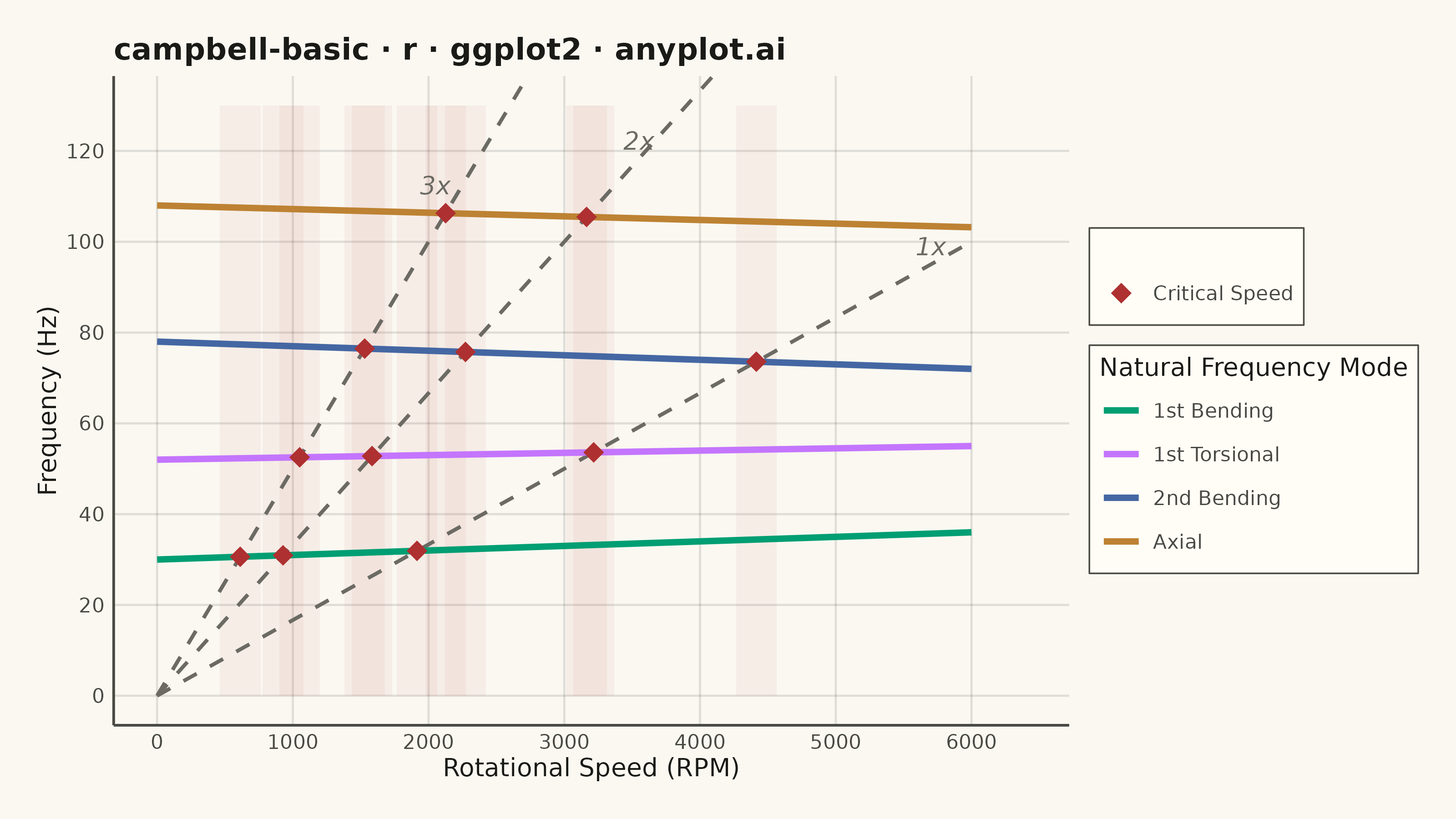
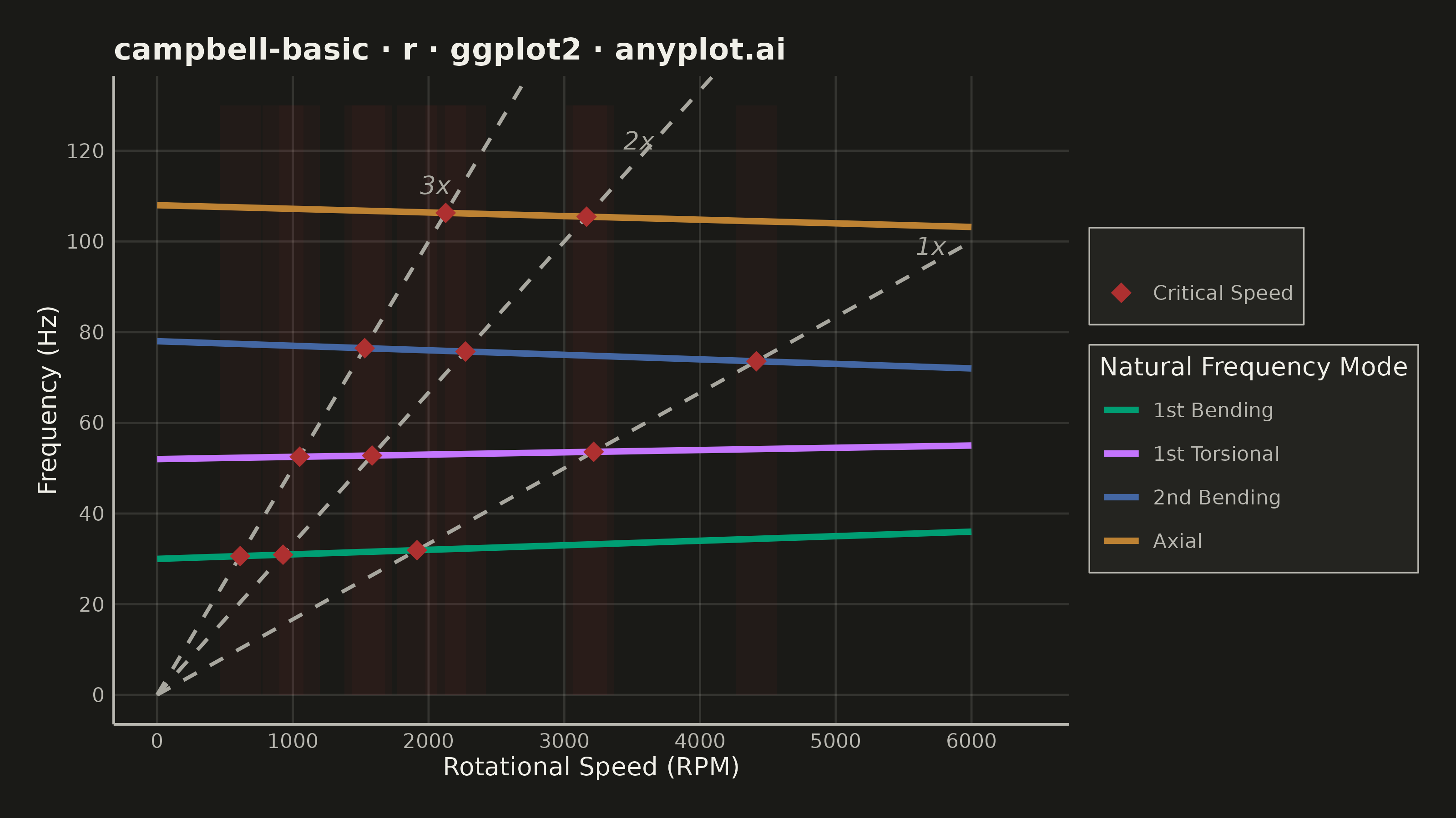
A Campbell Diagram (also called an interference diagram) plots natural frequencies against rotational speed to identify critical speeds and resonance conditions in rotating machinery. It overlays engine order excitation lines (diagonal lines from the origin) on top of natural frequency curves, with intersections marking critical speeds where resonance may occur. This visualization is essential for ensuring safe operating ranges in turbomachinery, automotive powertrains, and other rotating equipment.
#' anyplot.ai
#' campbell-basic: Campbell Diagram
#' Library: ggplot2 3.5.1 | R 4.4.1
#' Quality: 89/100 | Created: 2026-05-28

library(ggplot2)
library(ragg)

# Theme tokens
THEME       <- Sys.getenv("ANYPLOT_THEME", "light")
PAGE_BG     <- if (THEME == "light") "#FAF8F1" else "#1A1A17"
ELEVATED_BG <- if (THEME == "light") "#FFFDF6" else "#242420"
INK         <- if (THEME == "light") "#1A1A17" else "#F0EFE8"
INK_SOFT    <- if (THEME == "light") "#4A4A44" else "#B8B7B0"
INK_MUTED   <- if (THEME == "light") "#6B6A63" else "#A8A79F"
GRID        <- adjustcolor(INK, alpha.f = 0.12)

IMPRINT_PALETTE <- c("#009E73", "#C475FD", "#4467A3", "#BD8233")
CRITICAL_COLOR  <- "#AE3030"

# Rotational speed range: 0 to 6000 RPM (turbomachinery operating range)
speed <- seq(0, 6000, length.out = 100)

# Natural frequency modes (Hz) with slight gyroscopic speed dependence
mode_levels <- c("1st Bending", "1st Torsional", "2nd Bending", "Axial")
mode_data <- rbind(
  data.frame(speed = speed, frequency = 30 + 0.001 * speed,   mode = "1st Bending"),
  data.frame(speed = speed, frequency = 52 + 0.0005 * speed,  mode = "1st Torsional"),
  data.frame(speed = speed, frequency = 78 - 0.001 * speed,   mode = "2nd Bending"),
  data.frame(speed = speed, frequency = 108 - 0.0008 * speed, mode = "Axial")
)
mode_data$mode <- factor(mode_data$mode, levels = mode_levels)

# Engine order excitation lines (frequency = order * speed / 60)
order_data <- rbind(
  data.frame(speed = speed, frequency = 1 * speed / 60, order = "1x"),
  data.frame(speed = speed, frequency = 2 * speed / 60, order = "2x"),
  data.frame(speed = speed, frequency = 3 * speed / 60, order = "3x")
)

# Critical speed intersections: mode f = a + b*s, engine order f = n*s/60
# Setting equal: a + b*s = n*s/60 → s_crit = a / (n/60 - b)
y_max <- 130
mode_params <- list(
  list(a = 30,  b =  0.001),
  list(a = 52,  b =  0.0005),
  list(a = 78,  b = -0.001),
  list(a = 108, b = -0.0008)
)

critical_rows <- list()
for (n in 1:3) {
  for (m in mode_params) {
    denom  <- n / 60 - m$b
    s_crit <- m$a / denom
    f_crit <- n * s_crit / 60
    if (s_crit > 0 & s_crit <= 6000 & f_crit <= y_max) {
      critical_rows[[length(critical_rows) + 1]] <-
        data.frame(speed = s_crit, frequency = f_crit)
    }
  }
}
critical_pts <- do.call(rbind, critical_rows)

# Semi-transparent shading bands centered on each critical speed
zone_data <- data.frame(
  xmin = critical_pts$speed - 150,
  xmax = critical_pts$speed + 150,
  ymin = 0,
  ymax = y_max
)

# Engine order label positions — "3x" nudged extra to avoid Axial mode overlap
order_labels <- data.frame(
  speed     = c(5700, 3550, 2050),
  frequency = c(5700 / 60 + 4, 2 * 3550 / 60 + 4, 3 * 2050 / 60 + 10),
  label     = c("1x", "2x", "3x")
)

# Build plot
p <- ggplot() +
  geom_rect(
    data = zone_data,
    aes(xmin = xmin, xmax = xmax, ymin = ymin, ymax = ymax),
    fill = CRITICAL_COLOR, alpha = 0.05, inherit.aes = FALSE
  ) +
  geom_line(
    data = order_data,
    aes(x = speed, y = frequency, group = order),
    color = INK_MUTED, linewidth = 0.7, linetype = "dashed"
  ) +
  geom_line(
    data = mode_data,
    aes(x = speed, y = frequency, color = mode),
    linewidth = 1.2
  ) +
  geom_point(
    data = critical_pts,
    aes(x = speed, y = frequency, shape = "Critical Speed"),
    size = 3.5, color = CRITICAL_COLOR
  ) +
  geom_text(
    data = order_labels,
    aes(x = speed, y = frequency, label = label),
    color = INK_MUTED, size = 3.5, hjust = 0.5, fontface = "italic"
  ) +
  scale_color_manual(
    name   = "Natural Frequency Mode",
    values = setNames(IMPRINT_PALETTE, mode_levels)
  ) +
  scale_shape_manual(
    name   = "",
    values = c("Critical Speed" = 18)
  ) +
  scale_x_continuous(
    name   = "Rotational Speed (RPM)",
    breaks = seq(0, 6000, by = 1000)
  ) +
  scale_y_continuous(
    name   = "Frequency (Hz)",
    breaks = seq(0, 120, by = 20)
  ) +
  coord_cartesian(xlim = c(0, 6400), ylim = c(0, y_max)) +
  labs(title = "campbell-basic · r · ggplot2 · anyplot.ai") +
  theme_minimal(base_size = 8) +
  theme(
    plot.background   = element_rect(fill = PAGE_BG, color = PAGE_BG),
    panel.background  = element_rect(fill = PAGE_BG, color = NA),
    panel.grid.major  = element_line(color = GRID, linewidth = 0.4),
    panel.grid.minor  = element_blank(),
    panel.border      = element_blank(),
    axis.line         = element_line(color = INK_SOFT, linewidth = 0.5),
    axis.title        = element_text(color = INK,      size = 10),
    axis.text         = element_text(color = INK_SOFT, size = 8),
    plot.title        = element_text(color = INK,      size = 12, face = "bold"),
    legend.background = element_rect(fill = ELEVATED_BG, color = INK_SOFT,
                                     linewidth = 0.3),
    legend.text       = element_text(color = INK_SOFT, size = 8),
    legend.title      = element_text(color = INK,      size = 10),
    legend.position   = "right",
    plot.margin       = margin(15, 15, 15, 15)
  )

ggsave(
  filename = sprintf("plot-%s.png", THEME),
  plot     = p,
  device   = ragg::agg_png,
  width    = 8,
  height   = 4.5,
  units    = "in",
  dpi      = 400
)
Runnable source as JSON, for any HTTP client: https://api.anyplot.ai/specs/campbell-basic/ggplot2/code. Any spec id and library id listed in llms-full.txt fit the same URL shape; every URL below is complete and callable.
{
  "spec_id": "campbell-basic",
  "language": "r",
  "library": "ggplot2",
  "page": "https://anyplot.ai/campbell-basic/r/ggplot2",
  "hub": "https://anyplot.ai/campbell-basic",
  "code_json": "https://api.anyplot.ai/specs/campbell-basic/ggplot2/code",
  "spec_json": "https://api.anyplot.ai/specs/campbell-basic",
  "render_light_png": "https://storage.googleapis.com/anyplot-images/plots/campbell-basic/r/ggplot2/plot-light.png",
  "render_dark_png": "https://storage.googleapis.com/anyplot-images/plots/campbell-basic/r/ggplot2/plot-dark.png",
  "quality_score": 89.0,
  "license": "MIT",
  "guide": "https://anyplot.ai/llms.txt"
}
Part of Campbell Diagram on anyplot.ai.