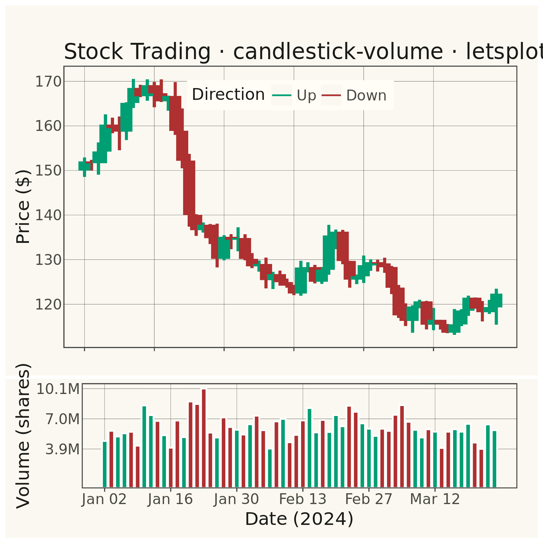
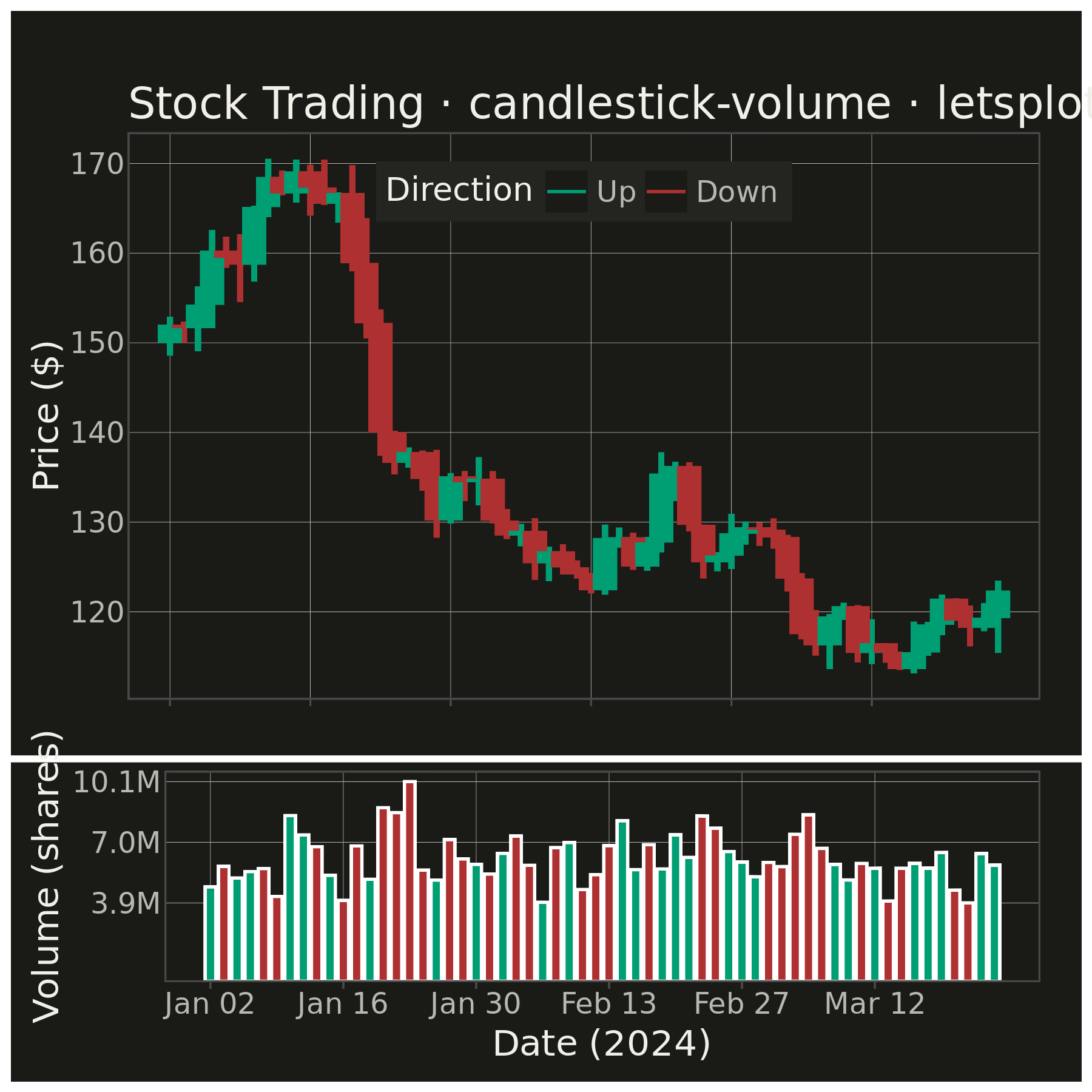
A professional candlestick chart combining OHLC (open, high, low, close) price data with volume bars in a synchronized lower pane. The dual-pane layout presents price action in the main chart with corresponding trading volume below, sharing a common time axis. This format is the standard for technical analysis platforms, enabling traders to correlate price movements with trading activity and identify volume-confirmed trends or reversals.
""" anyplot.ai
candlestick-volume: Stock Candlestick Chart with Volume
Library: letsplot 4.9.0 | Python 3.13.13
Quality: 90/100 | Updated: 2026-05-16
"""

import os

import numpy as np
import pandas as pd
from lets_plot import *


LetsPlot.setup_html()

THEME = os.getenv("ANYPLOT_THEME", "light")
PAGE_BG = "#FAF8F1" if THEME == "light" else "#1A1A17"
ELEVATED_BG = "#FFFDF6" if THEME == "light" else "#242420"
INK = "#1A1A17" if THEME == "light" else "#F0EFE8"
INK_SOFT = "#4A4A44" if THEME == "light" else "#B8B7B0"

# Data - 60 trading days of synthetic stock data
np.random.seed(42)
n_days = 60
dates = pd.date_range("2024-01-02", periods=n_days, freq="B")

# Generate realistic price movement with more dramatic reversals
returns = np.random.normal(0.001, 0.025, n_days)
returns[15] = -0.08  # Dramatic drop
returns[35] = 0.06  # Strong bounce
returns[45] = -0.05  # Another reversal
close_prices = 150 * np.cumprod(1 + returns)

# Generate OHLC from close prices
open_prices = np.roll(close_prices, 1)
open_prices[0] = 150
high_prices = np.maximum(open_prices, close_prices) * (1 + np.abs(np.random.normal(0, 0.012, n_days)))
low_prices = np.minimum(open_prices, close_prices) * (1 - np.abs(np.random.normal(0, 0.012, n_days)))

# Generate volume with correlation to price movement
base_volume = 5_000_000
volatility = np.abs(close_prices - open_prices) / open_prices
volume = base_volume * (1 + volatility * 10 + np.random.uniform(-0.3, 0.3, n_days))
volume = volume.astype(int)

# Determine up/down days for coloring
direction = ["Up" if c >= o else "Down" for c, o in zip(close_prices, open_prices)]

# Create date labels for x-axis (show every 10 trading days)
date_labels = [d.strftime("%b %d") for d in dates]
date_breaks = list(range(0, n_days, 10))
date_tick_labels = [date_labels[i] for i in date_breaks]

df = pd.DataFrame(
    {
        "date": dates,
        "date_idx": range(n_days),
        "date_label": date_labels,
        "open": open_prices,
        "high": high_prices,
        "low": low_prices,
        "close": close_prices,
        "volume": volume,
        "direction": direction,
    }
)

# Colorblind-safe colors (first series Okabe-Ito, second is orange)
color_up = "#009E73"
color_down = "#AE3030"  # imprint red — down days

# Create volume breaks and labels (inline formatting)
vol_min, vol_max = df["volume"].min(), df["volume"].max()
vol_breaks = [int(vol_min), int((vol_min + vol_max) / 2), int(vol_max)]
vol_labels = [f"{v / 1_000_000:.1f}M" if v >= 1_000_000 else f"{v / 1_000:.0f}K" for v in vol_breaks]

# Theme-adaptive styling
anyplot_theme = theme(
    plot_background=element_rect(fill=PAGE_BG, color=PAGE_BG),
    panel_background=element_rect(fill=PAGE_BG),
    panel_grid_major=element_line(color=INK_SOFT, size=0.25),
    panel_grid_minor=element_blank(),
    axis_title=element_text(color=INK, size=20),
    axis_text=element_text(color=INK_SOFT, size=16),
    axis_line=element_line(color=INK_SOFT, size=0.3),
    plot_title=element_text(color=INK, size=24),
    legend_background=element_rect(fill=ELEVATED_BG, color=INK_SOFT),
    legend_text=element_text(color=INK_SOFT, size=16),
    legend_title=element_text(color=INK, size=18),
)

# Create candlestick chart (main pane)
candle_plot = (
    ggplot(df)
    # Wicks (high-low lines) - thicker for visibility
    + geom_segment(aes(x="date_idx", xend="date_idx", y="low", yend="high", color="direction"), size=1.5)
    # Bodies (open-close rectangles)
    + geom_segment(aes(x="date_idx", xend="date_idx", y="open", yend="close", color="direction"), size=6.0)
    + scale_color_manual(values={"Up": color_up, "Down": color_down}, name="Direction")
    + scale_x_continuous(breaks=date_breaks, labels=date_tick_labels)
    + labs(title="Stock Trading · candlestick-volume · letsplot · anyplot.ai", y="Price ($)", x="")
    + anyplot_theme
    + theme(
        axis_text_x=element_blank(),
        legend_position=[0.5, 0.95],
        legend_justification=[0.5, 1.0],
        legend_direction="horizontal",
        plot_margin=[40, 20, 2, 10],
    )
    + ggsize(1600, 630)
)

# Volume chart (lower pane)
volume_plot = (
    ggplot(df)
    + geom_bar(aes(x="date_idx", y="volume", fill="direction"), stat="identity", width=0.8)
    + scale_fill_manual(values={"Up": color_up, "Down": color_down}, name="Direction")
    + scale_x_continuous(breaks=date_breaks, labels=date_tick_labels)
    + scale_y_continuous(breaks=vol_breaks, labels=vol_labels)
    + labs(x="Date (2024)", y="Volume (shares)")
    + anyplot_theme
    + theme(legend_position="none", plot_margin=[2, 20, 10, 10])
    + ggsize(1600, 270)
)

# Use gggrid for dual-pane layout with tighter spacing
combined = gggrid([candle_plot, volume_plot], ncol=1, heights=[0.7, 0.3])

# Save outputs
ggsave(combined, f"plot-{THEME}.png", scale=3, path=".")
ggsave(combined, f"plot-{THEME}.html", path=".")
Runnable source as JSON, for any HTTP client: https://api.anyplot.ai/specs/candlestick-volume/letsplot/code. Any spec id and library id listed in llms-full.txt fit the same URL shape; every URL below is complete and callable.
{
  "spec_id": "candlestick-volume",
  "language": "python",
  "library": "letsplot",
  "page": "https://anyplot.ai/candlestick-volume/python/letsplot",
  "hub": "https://anyplot.ai/candlestick-volume",
  "code_json": "https://api.anyplot.ai/specs/candlestick-volume/letsplot/code",
  "spec_json": "https://api.anyplot.ai/specs/candlestick-volume",
  "render_light_png": "https://storage.googleapis.com/anyplot-images/plots/candlestick-volume/python/letsplot/plot-light.png",
  "render_dark_png": "https://storage.googleapis.com/anyplot-images/plots/candlestick-volume/python/letsplot/plot-dark.png",
  "interactive_light_html": "https://storage.googleapis.com/anyplot-images/plots/candlestick-volume/python/letsplot/plot-light.html",
  "interactive_dark_html": "https://storage.googleapis.com/anyplot-images/plots/candlestick-volume/python/letsplot/plot-dark.html",
  "quality_score": 90.0,
  "license": "MIT",
  "guide": "https://anyplot.ai/llms.txt"
}
Part of Stock Candlestick Chart with Volume on anyplot.ai.