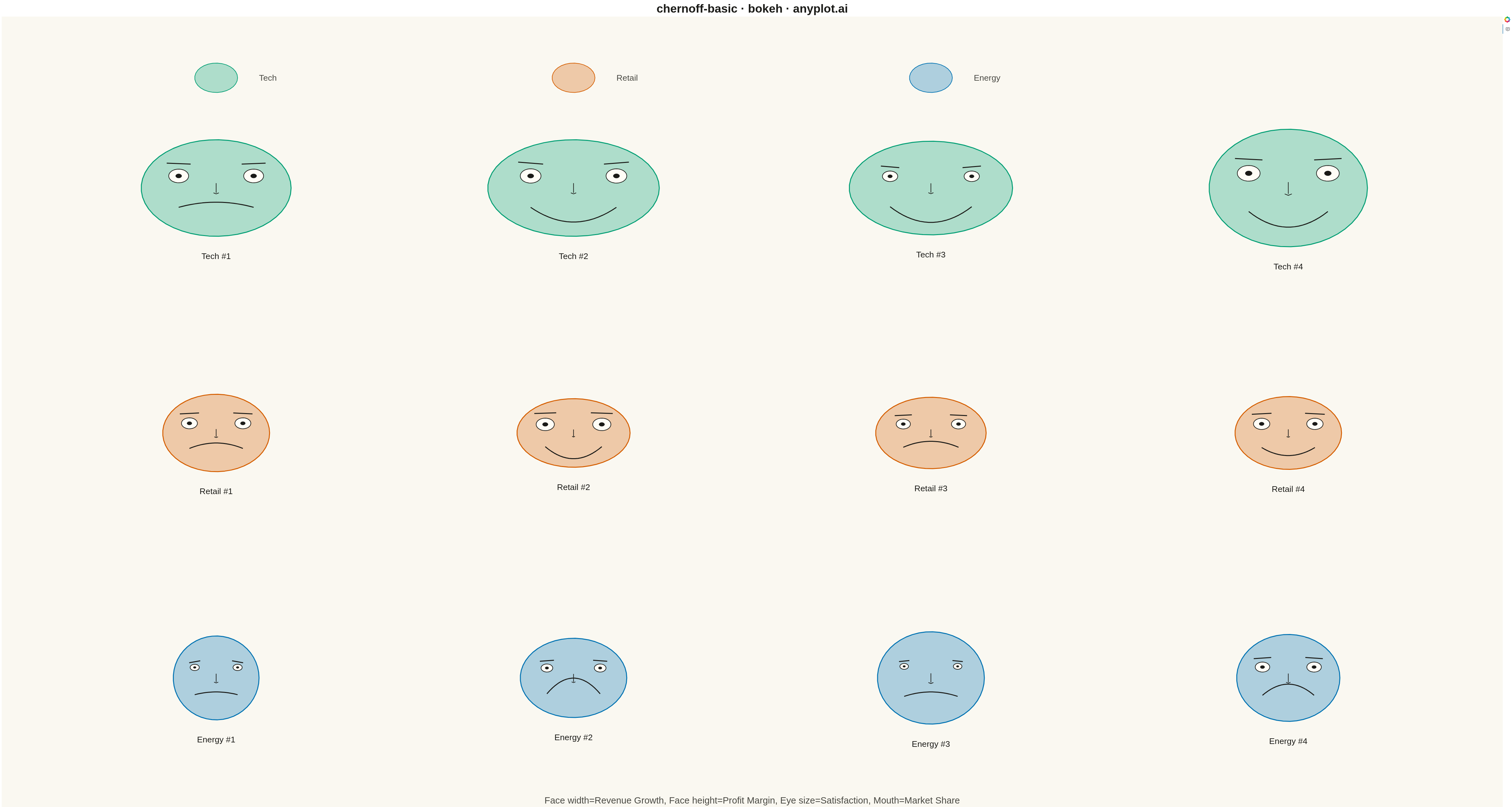
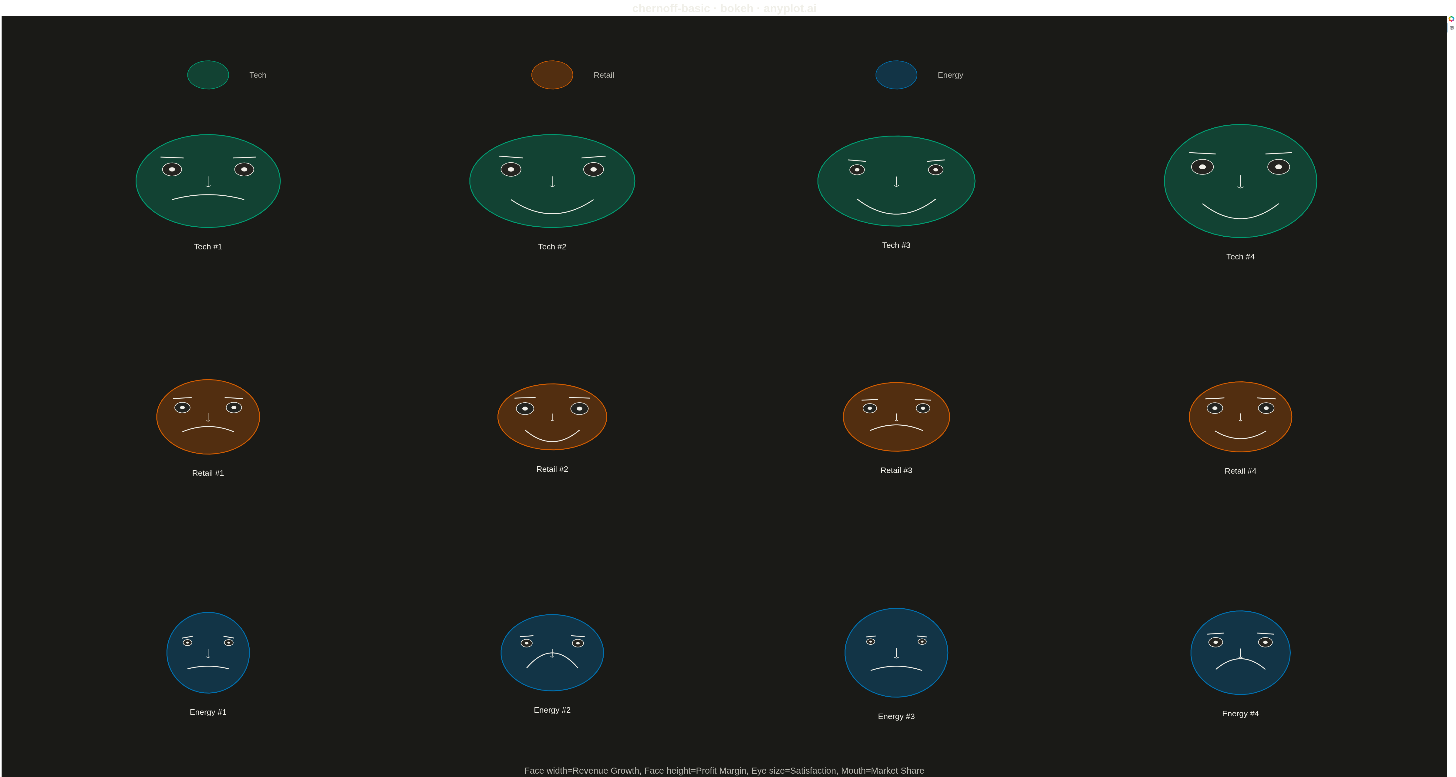
Chernoff faces visualize multivariate data by mapping each variable to a facial feature (eye size, mouth curvature, face width, nose length, etc.), transforming each observation into a unique cartoon face. This technique leverages humans' innate ability to recognize and distinguish faces, making it easier to identify patterns, clusters, and outliers across multiple dimensions simultaneously.
""" anyplot.ai
chernoff-basic: Chernoff Faces for Multivariate Data
Library: bokeh 3.9.0 | Python 3.13.13
Quality: 79/100 | Updated: 2026-05-15
"""

import numpy as np
from bokeh.io import export_png
from bokeh.models import ColumnDataSource, HoverTool, Label
from bokeh.plotting import figure


# Generate synthetic company performance data (4 metrics for 12 companies)
# Metrics: Revenue Growth, Profit Margin, Customer Satisfaction, Market Share
np.random.seed(42)

# Three company sectors with different profiles
sectors = ["Tech", "Retail", "Energy"]
sector_idx = np.array([0, 0, 0, 0, 1, 1, 1, 1, 2, 2, 2, 2])

# Tech companies: high growth, high margin
tech_data = np.column_stack(
    [
        np.random.uniform(0.6, 1.0, 4),  # Revenue Growth
        np.random.uniform(0.5, 0.9, 4),  # Profit Margin
        np.random.uniform(0.6, 0.95, 4),  # Customer Satisfaction
        np.random.uniform(0.3, 0.7, 4),  # Market Share
    ]
)

# Retail companies: moderate growth, moderate margin
retail_data = np.column_stack(
    [
        np.random.uniform(0.2, 0.5, 4),  # Revenue Growth
        np.random.uniform(0.15, 0.4, 4),  # Profit Margin
        np.random.uniform(0.5, 0.8, 4),  # Customer Satisfaction
        np.random.uniform(0.4, 0.8, 4),  # Market Share
    ]
)

# Energy companies: low growth, variable margin
energy_data = np.column_stack(
    [
        np.random.uniform(0.05, 0.3, 4),  # Revenue Growth
        np.random.uniform(0.3, 0.6, 4),  # Profit Margin
        np.random.uniform(0.3, 0.6, 4),  # Customer Satisfaction
        np.random.uniform(0.5, 0.9, 4),  # Market Share
    ]
)

data = np.vstack([tech_data, retail_data, energy_data])

# Normalize each feature to 0-1
data_norm = (data - data.min(axis=0)) / (data.max(axis=0) - data.min(axis=0) + 1e-10)

# Colors for sectors
colors = ["#306998", "#FFD43B", "#8B4513"]

# Store face center data for hover tooltips using ColumnDataSource
face_centers_x = []
face_centers_y = []
face_labels = []
face_revenue = []
face_margin = []
face_satisfaction = []
face_market_share = []

# Create figure with 4x3 grid for 12 faces
p = figure(
    width=4800,
    height=2700,
    title="chernoff-basic · bokeh · pyplots.ai",
    x_range=(-0.1, 4.1),
    y_range=(-0.2, 3.2),
    tools="",
)

# Style
p.title.text_font_size = "32pt"
p.title.align = "center"
p.xaxis.visible = False
p.yaxis.visible = False
p.xgrid.visible = False
p.ygrid.visible = False
p.outline_line_color = None
p.background_fill_color = "#FAFAFA"

# Draw faces in a 4x3 grid (inline, no helper function)
face_size = 0.4
for i, (features, sec_idx) in enumerate(zip(data_norm, sector_idx, strict=True)):
    col = i % 4
    row = 2 - i // 4  # Start from top row
    cx = col + 0.5
    cy = row + 0.5
    color = colors[sec_idx]
    label_text = f"{sectors[sec_idx]} #{i % 4 + 1}"

    # Store data for hover tooltip
    face_centers_x.append(cx)
    face_centers_y.append(cy)
    face_labels.append(label_text)
    face_revenue.append(f"{data[i, 0] * 100:.1f}%")
    face_margin.append(f"{data[i, 1] * 100:.1f}%")
    face_satisfaction.append(f"{data[i, 2] * 100:.1f}%")
    face_market_share.append(f"{data[i, 3] * 100:.1f}%")

    # Features mapping:
    # - revenue_growth (features[0]) -> face width
    # - profit_margin (features[1]) -> face height
    # - customer_satisfaction (features[2]) -> eye size
    # - market_share (features[3]) -> mouth curvature
    face_width = (0.3 + features[0] * 0.3) * face_size
    face_height = (0.35 + features[1] * 0.25) * face_size
    eye_size = (0.03 + features[2] * 0.05) * face_size
    mouth_curve = features[3]

    # Draw face outline (ellipse approximation using patches)
    theta = np.linspace(0, 2 * np.pi, 50)
    face_x = cx + face_width * np.cos(theta)
    face_y = cy + face_height * np.sin(theta)
    p.patch(face_x, face_y, fill_color=color, fill_alpha=0.3, line_color=color, line_width=3)

    # Draw eyes
    eye_spacing = face_width * 0.5
    eye_y = cy + face_height * 0.25
    eye_theta = np.linspace(0, 2 * np.pi, 30)

    # Left eye
    left_eye_x = cx - eye_spacing
    left_ex = left_eye_x + eye_size * np.cos(eye_theta)
    left_ey = eye_y + eye_size * np.sin(eye_theta)
    p.patch(left_ex, left_ey, fill_color="white", line_color="#333333", line_width=2)

    # Left pupil
    pupil_size = eye_size * 0.5
    left_px = left_eye_x + pupil_size * np.cos(eye_theta) * 0.6
    left_py = eye_y + pupil_size * np.sin(eye_theta) * 0.6
    p.patch(left_px, left_py, fill_color="#333333", line_color="#333333")

    # Right eye
    right_eye_x = cx + eye_spacing
    right_ex = right_eye_x + eye_size * np.cos(eye_theta)
    right_ey = eye_y + eye_size * np.sin(eye_theta)
    p.patch(right_ex, right_ey, fill_color="white", line_color="#333333", line_width=2)

    # Right pupil
    right_px = right_eye_x + pupil_size * np.cos(eye_theta) * 0.6
    right_py = eye_y + pupil_size * np.sin(eye_theta) * 0.6
    p.patch(right_px, right_py, fill_color="#333333", line_color="#333333")

    # Draw eyebrows
    brow_y = eye_y + eye_size * 1.8
    brow_width = eye_size * 1.2
    eyebrow_slant = (features[0] - 0.5) * 0.02 * face_size

    p.line(
        [left_eye_x - brow_width, left_eye_x + brow_width],
        [brow_y + eyebrow_slant, brow_y - eyebrow_slant],
        line_color="#333333",
        line_width=3,
    )
    p.line(
        [right_eye_x - brow_width, right_eye_x + brow_width],
        [brow_y - eyebrow_slant, brow_y + eyebrow_slant],
        line_color="#333333",
        line_width=3,
    )

    # Draw nose
    nose_length = (0.02 + features[1] * 0.03) * face_size
    nose_y_top = cy + face_height * 0.1
    nose_y_bottom = cy - face_height * 0.1
    p.line([cx, cx], [nose_y_top, nose_y_bottom], line_color="#333333", line_width=2)
    p.line(
        [cx - nose_length * 0.5, cx, cx + nose_length * 0.5],
        [nose_y_bottom, nose_y_bottom - nose_length * 0.3, nose_y_bottom],
        line_color="#333333",
        line_width=2,
    )

    # Draw mouth (curved based on market_share)
    mouth_y = cy - face_height * 0.4
    mouth_width = face_width * 0.5
    mouth_x = np.linspace(cx - mouth_width, cx + mouth_width, 20)
    curve_amount = (mouth_curve - 0.5) * 0.08 * face_size
    mouth_y_curve = mouth_y + curve_amount * (1 - ((mouth_x - cx) / mouth_width) ** 2) * 4
    p.line(mouth_x, mouth_y_curve, line_color="#333333", line_width=3)

    # Add label below face
    label_obj = Label(
        x=cx,
        y=cy - face_height - 0.1,
        text=label_text,
        text_align="center",
        text_font_size="20pt",
        text_color="#333333",
    )
    p.add_layout(label_obj)

# Create ColumnDataSource for hover tooltips (Bokeh-specific feature)
hover_source = ColumnDataSource(
    data={
        "x": face_centers_x,
        "y": face_centers_y,
        "label": face_labels,
        "revenue": face_revenue,
        "margin": face_margin,
        "satisfaction": face_satisfaction,
        "market_share": face_market_share,
    }
)

# Add invisible scatter for hover interaction
hover_renderer = p.scatter("x", "y", source=hover_source, size=80, fill_alpha=0, line_alpha=0)

# Add HoverTool for interactivity (distinctive Bokeh feature)
hover_tool = HoverTool(
    renderers=[hover_renderer],
    tooltips=[
        ("Company", "@label"),
        ("Revenue Growth", "@revenue"),
        ("Profit Margin", "@margin"),
        ("Satisfaction", "@satisfaction"),
        ("Market Share", "@market_share"),
    ],
)
p.add_tools(hover_tool)

# Add legend manually using patches and labels (positioned below grid)
legend_y_base = 2.95
legend_x_positions = [0.5, 1.5, 2.5]
for i, (name, color) in enumerate(zip(sectors, colors, strict=True)):
    lx_center = legend_x_positions[i]
    theta = np.linspace(0, 2 * np.pi, 30)
    lx = lx_center + 0.06 * np.cos(theta)
    ly = legend_y_base + 0.06 * np.sin(theta)
    p.patch(lx, ly, fill_color=color, fill_alpha=0.3, line_color=color, line_width=2)
    legend_label = Label(
        x=lx_center + 0.12, y=legend_y_base - 0.02, text=name, text_font_size="20pt", text_color="#333333"
    )
    p.add_layout(legend_label)

# Add subtitle with feature mapping explanation (increased font size)
subtitle = Label(
    x=2.0,
    y=-0.02,
    text="Face width=Revenue Growth, Face height=Profit Margin, Eye size=Satisfaction, Mouth=Market Share",
    text_align="center",
    text_font_size="22pt",
    text_color="#666666",
)
p.add_layout(subtitle)

# Save
export_png(p, filename="plot.png")
Runnable source as JSON, for any HTTP client: https://api.anyplot.ai/specs/chernoff-basic/bokeh/code. Any spec id and library id listed in llms-full.txt fit the same URL shape; every URL below is complete and callable.
{
  "spec_id": "chernoff-basic",
  "language": "python",
  "library": "bokeh",
  "page": "https://anyplot.ai/chernoff-basic/python/bokeh",
  "hub": "https://anyplot.ai/chernoff-basic",
  "code_json": "https://api.anyplot.ai/specs/chernoff-basic/bokeh/code",
  "spec_json": "https://api.anyplot.ai/specs/chernoff-basic",
  "render_light_png": "https://storage.googleapis.com/anyplot-images/plots/chernoff-basic/python/bokeh/plot-light.png",
  "render_dark_png": "https://storage.googleapis.com/anyplot-images/plots/chernoff-basic/python/bokeh/plot-dark.png",
  "interactive_light_html": "https://storage.googleapis.com/anyplot-images/plots/chernoff-basic/python/bokeh/plot-light.html",
  "interactive_dark_html": "https://storage.googleapis.com/anyplot-images/plots/chernoff-basic/python/bokeh/plot-dark.html",
  "quality_score": 79.0,
  "license": "MIT",
  "guide": "https://anyplot.ai/llms.txt"
}
Part of Chernoff Faces for Multivariate Data on anyplot.ai.