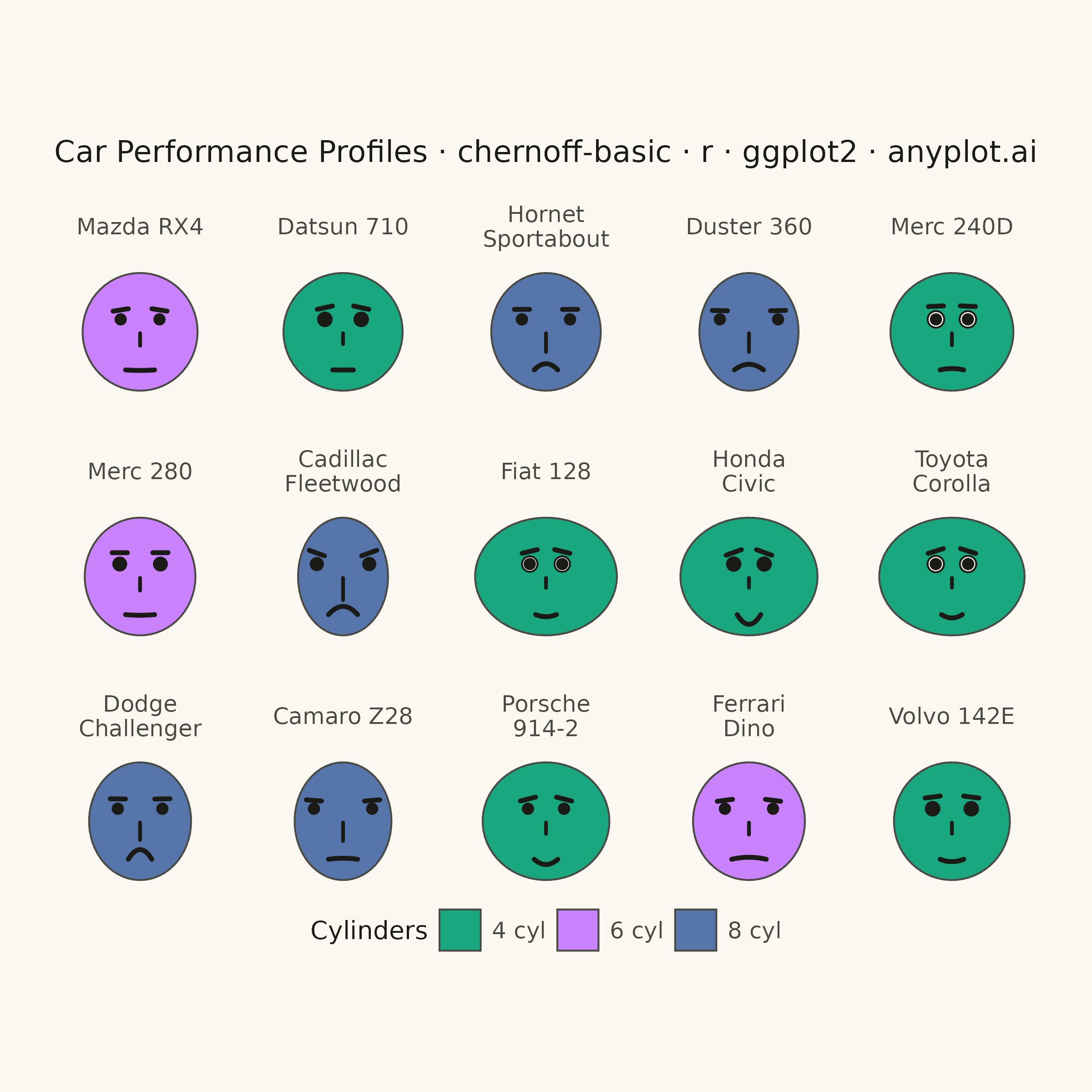
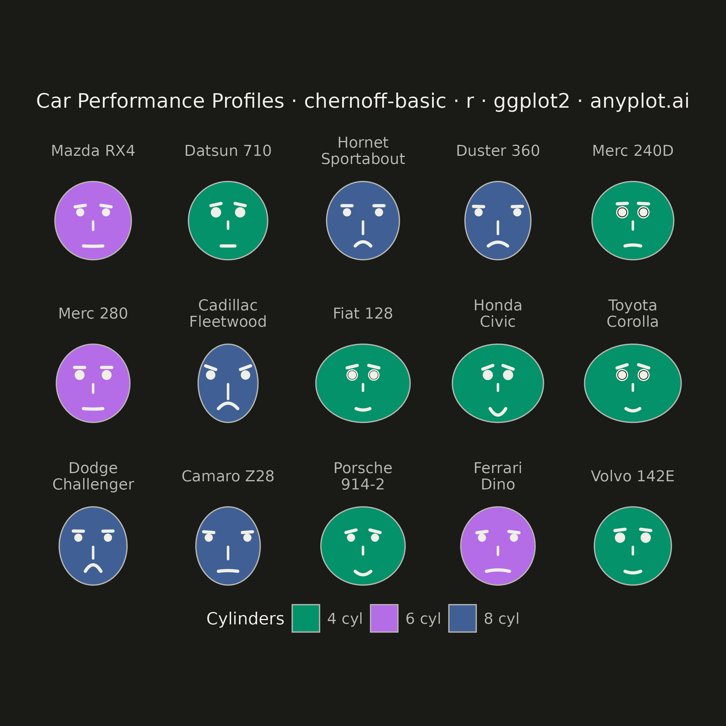
The same plot in 14 other libraries — Python: Altair, Bokeh, lets-plot, Matplotlib, Plotly, plotnine, Pygal, Seaborn; Julia: Makie.jl; JavaScript: Chart.js, D3.js, Apache ECharts, Highcharts, MUI X Charts. Compare all 15 side by side: Chernoff Faces for Multivariate Data in Python, R, Julia and JavaScript.
Chernoff faces visualize multivariate data by mapping each variable to a facial feature (eye size, mouth curvature, face width, nose length, etc.), transforming each observation into a unique cartoon face. This technique leverages humans' innate ability to recognize and distinguish faces, making it easier to identify patterns, clusters, and outliers across multiple dimensions simultaneously.
#' anyplot.ai
#' chernoff-basic: Chernoff Faces for Multivariate Data
#' Library: ggplot2 3.5.1 | R 4.4.1
#' Quality: 93/100 | Created: 2026-09-02

library(ggplot2)
library(dplyr)
library(tibble)
library(scales)
library(ragg)

set.seed(42)

# --- Theme tokens ------------------------------------------------------------
THEME       <- Sys.getenv("ANYPLOT_THEME", "light")
PAGE_BG     <- if (THEME == "light") "#FAF8F1" else "#1A1A17"
INK         <- if (THEME == "light") "#1A1A17" else "#F0EFE8"
INK_SOFT    <- if (THEME == "light") "#4A4A44" else "#B8B7B0"
IMPRINT_PALETTE <- c("#009E73", "#C475FD", "#4467A3", "#BD8233",
                     "#AE3030", "#2ABCCD", "#954477", "#99B314")

# --- Data: mtcars performance metrics per model -------------------------------
cars <- c(
  "Mazda RX4", "Datsun 710", "Hornet Sportabout", "Duster 360",
  "Merc 240D", "Merc 280", "Cadillac Fleetwood", "Fiat 128",
  "Honda Civic", "Toyota Corolla", "Dodge Challenger", "Camaro Z28",
  "Porsche 914-2", "Ferrari Dino", "Volvo 142E"
)

faces <- rownames_to_column(mtcars, "car") |>
  filter(car %in% cars) |>
  mutate(
    car       = factor(car, levels = cars),
    cyl_group = factor(cyl, levels = c(4, 6, 8),
                        labels = c("4 cyl", "6 cyl", "8 cyl")),
    # Each performance metric is rescaled onto its own facial-feature range
    face_width  = rescale(mpg,  to = c(0.65, 1.05)),
    eye_size    = rescale(qsec, to = c(0.05, 0.12)),
    eye_spacing = rescale(hp,   to = c(0.22, 0.42)),
    brow_slant  = rescale(wt,   to = c(20, -20)),
    nose_length = rescale(disp, to = c(0.14, 0.32)),
    mouth_curve = rescale(drat, to = c(-1, 1)),
    mouth_width = rescale(carb, to = c(0.30, 0.50))
  ) |>
  arrange(car)

# --- Facial-feature geometry helpers ------------------------------------------
ellipse_pts <- function(cx, cy, rx, ry, n = 60) {
  t <- seq(0, 2 * pi, length.out = n)
  tibble(x = cx + rx * cos(t), y = cy + ry * sin(t))
}

mouth_pts <- function(cx, cy, half_width, curvature, amp = 0.14, n = 24) {
  t <- seq(-1, 1, length.out = n)
  tibble(x = cx + t * half_width, y = cy + curvature * amp * (t^2 - 1))
}

# --- Build one face's geometry per row, then stack into shared layers ---------
n_faces   <- nrow(faces)
brow_half <- 0.11
eye_y     <- 0.18

outline_list  <- vector("list", n_faces)
eyes_list     <- vector("list", n_faces)
pupils_list   <- vector("list", n_faces)
eyebrows_list <- vector("list", n_faces)
nose_list     <- vector("list", n_faces)
mouth_list    <- vector("list", n_faces)

for (i in seq_len(n_faces)) {
  row <- faces[i, ]

  outline_list[[i]] <- bind_cols(
    car = row$car, cyl_group = row$cyl_group,
    ellipse_pts(0, 0, row$face_width, 0.85)
  )

  eyes_list[[i]] <- bind_rows(
    bind_cols(car = row$car, side = "left",
              ellipse_pts(-row$eye_spacing, eye_y, row$eye_size, row$eye_size, n = 28)),
    bind_cols(car = row$car, side = "right",
              ellipse_pts( row$eye_spacing, eye_y, row$eye_size, row$eye_size, n = 28))
  )

  pupils_list[[i]] <- tibble(
    car = row$car,
    x   = c(-row$eye_spacing, row$eye_spacing),
    y   = c(eye_y, eye_y)
  )

  slant  <- row$brow_slant * pi / 180
  dy     <- brow_half * tan(slant)
  brow_y <- eye_y + row$eye_size + 0.07
  eyebrows_list[[i]] <- tibble(
    car  = row$car,
    x    = c(-row$eye_spacing - brow_half, row$eye_spacing - brow_half),
    xend = c(-row$eye_spacing + brow_half, row$eye_spacing + brow_half),
    y    = c(brow_y - dy, brow_y + dy),
    yend = c(brow_y + dy, brow_y - dy)
  )

  nose_list[[i]] <- tibble(
    car = row$car, x = 0, xend = 0,
    y = -0.02, yend = -0.02 - row$nose_length
  )

  mouth_list[[i]] <- bind_cols(
    car = row$car,
    mouth_pts(0, -0.55, row$mouth_width / 2, row$mouth_curve)
  )
}

outline_df  <- bind_rows(outline_list)
eyes_df     <- bind_rows(eyes_list)
pupils_df   <- bind_rows(pupils_list)
eyebrows_df <- bind_rows(eyebrows_list)
nose_df     <- bind_rows(nose_list)
mouth_df    <- bind_rows(mouth_list)

# --- Plot ----------------------------------------------------------------------
title_text     <- "Car Performance Profiles · chernoff-basic · r · ggplot2 · anyplot.ai"
title_fontsize <- round(12 * min(1, 67 / nchar(title_text)))

p <- ggplot() +
  geom_polygon(data = outline_df, aes(x, y, group = car, fill = cyl_group),
               color = INK_SOFT, linewidth = 0.35, alpha = 0.9) +
  geom_polygon(data = eyes_df, aes(x, y, group = interaction(car, side)),
               fill = PAGE_BG, color = INK, linewidth = 0.35) +
  geom_point(data = pupils_df, aes(x, y), color = INK, size = 1.6) +
  geom_segment(data = eyebrows_df, aes(x = x, xend = xend, y = y, yend = yend),
               color = INK, linewidth = 0.9, lineend = "round") +
  geom_segment(data = nose_df, aes(x = x, xend = xend, y = y, yend = yend),
               color = INK, linewidth = 0.7, lineend = "round") +
  geom_path(data = mouth_df, aes(x, y, group = car),
            color = INK, linewidth = 0.9, lineend = "round") +
  scale_fill_manual(values = IMPRINT_PALETTE[1:3], name = "Cylinders") +
  coord_equal(xlim = c(-1.15, 1.15), ylim = c(-1.05, 1.05), expand = FALSE) +
  facet_wrap(~ car, ncol = 5, labeller = label_wrap_gen(width = 11)) +
  labs(title = title_text) +
  theme_void(base_size = 8) +
  theme(
    plot.background   = element_rect(fill = PAGE_BG, color = PAGE_BG),
    panel.background  = element_rect(fill = PAGE_BG, color = NA),
    panel.spacing     = unit(1.2, "lines"),
    plot.title        = element_text(color = INK, size = title_fontsize, hjust = 0.5,
                                      margin = margin(b = 14)),
    strip.text        = element_text(color = INK_SOFT, size = 9, lineheight = 0.9,
                                      margin = margin(b = 4)),
    legend.position    = "bottom",
    legend.title       = element_text(color = INK, size = 10),
    legend.text        = element_text(color = INK_SOFT, size = 9),
    legend.background  = element_rect(fill = PAGE_BG, color = NA),
    legend.key         = element_rect(fill = PAGE_BG, color = NA),
    plot.margin        = margin(20, 24, 20, 24)
  )

# --- Save ------------------------------------------------------------------
ggsave(
  filename = sprintf("plot-%s.png", THEME),
  plot     = p,
  device   = ragg::agg_png,
  width    = 6,
  height   = 6,
  units    = "in",
  dpi      = 400
)
Runnable source as JSON, for any HTTP client: https://api.anyplot.ai/specs/chernoff-basic/ggplot2/code. Any spec id and library id listed in llms-full.txt fit the same URL shape; every URL below is complete and callable.
{
  "spec_id": "chernoff-basic",
  "language": "r",
  "library": "ggplot2",
  "page": "https://anyplot.ai/chernoff-basic/r/ggplot2",
  "hub": "https://anyplot.ai/chernoff-basic",
  "code_json": "https://api.anyplot.ai/specs/chernoff-basic/ggplot2/code",
  "spec_json": "https://api.anyplot.ai/specs/chernoff-basic",
  "render_light_png": "https://storage.googleapis.com/anyplot-images/plots/chernoff-basic/r/ggplot2/plot-light.png",
  "render_dark_png": "https://storage.googleapis.com/anyplot-images/plots/chernoff-basic/r/ggplot2/plot-dark.png",
  "quality_score": 93.0,
  "license": "MIT",
  "guide": "https://anyplot.ai/llms.txt"
}
Part of Chernoff Faces for Multivariate Data on anyplot.ai.