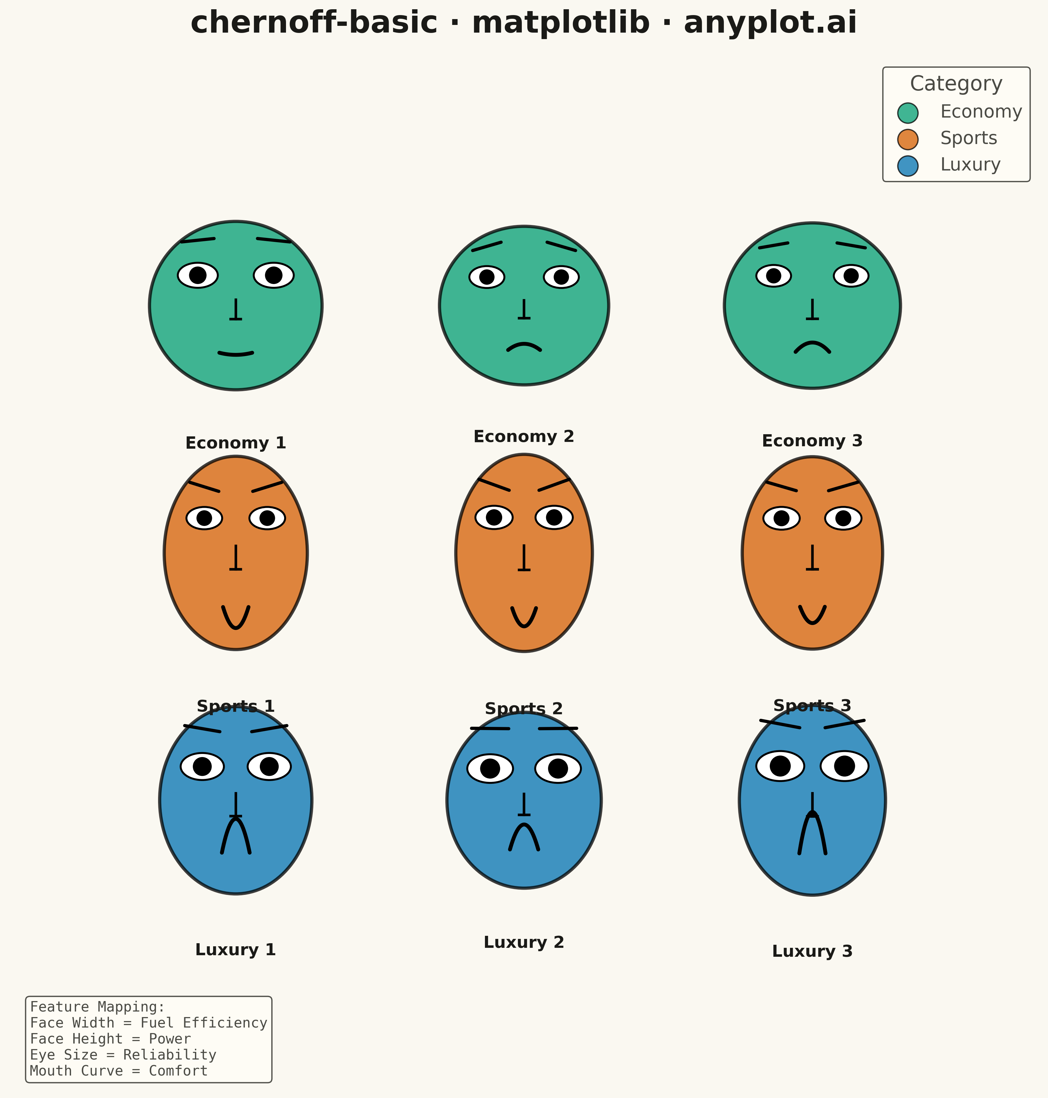
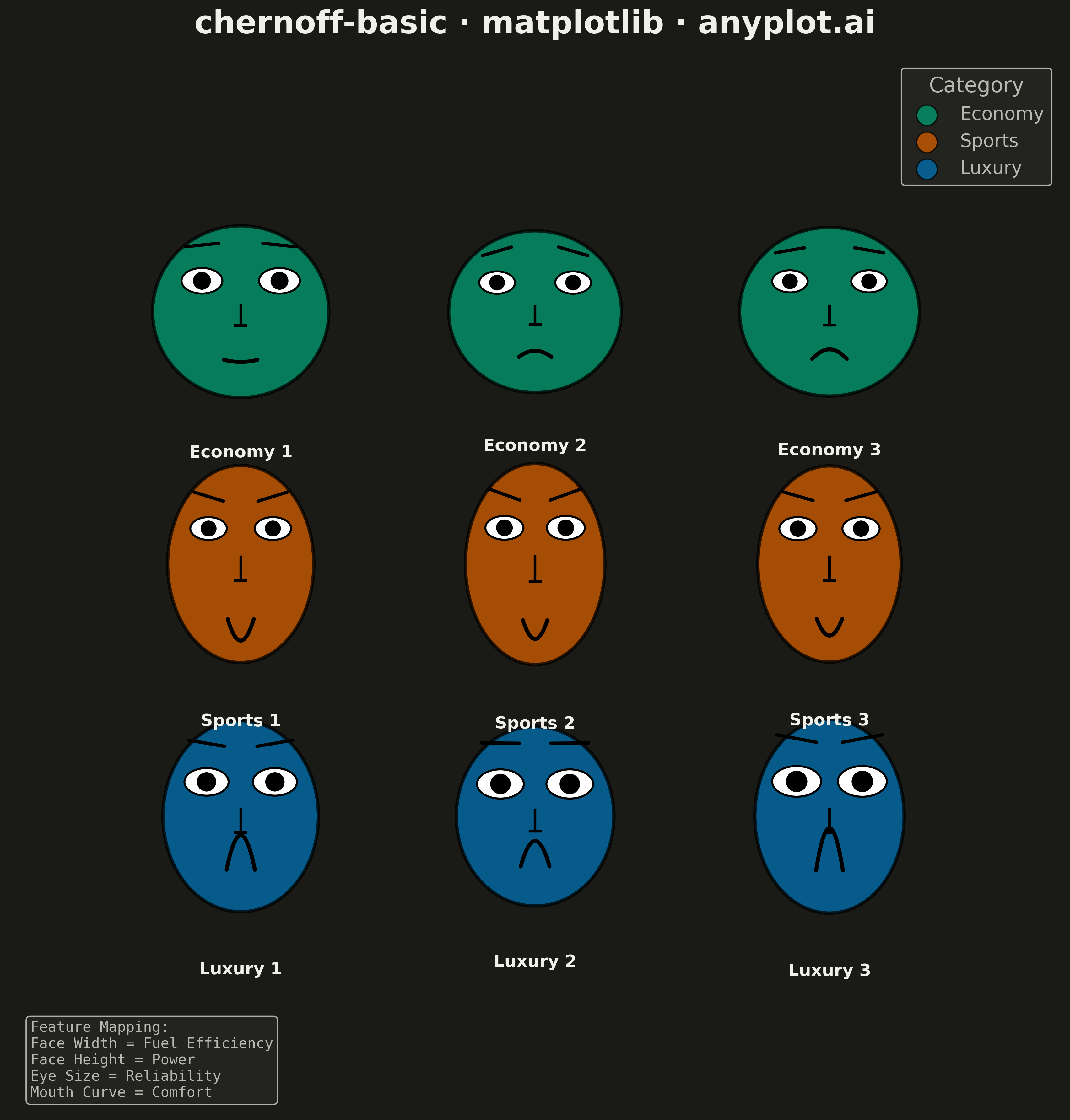
Chernoff faces visualize multivariate data by mapping each variable to a facial feature (eye size, mouth curvature, face width, nose length, etc.), transforming each observation into a unique cartoon face. This technique leverages humans' innate ability to recognize and distinguish faces, making it easier to identify patterns, clusters, and outliers across multiple dimensions simultaneously.
""" anyplot.ai
chernoff-basic: Chernoff Faces for Multivariate Data
Library: matplotlib 3.10.9 | Python 3.13.13
Quality: 88/100 | Updated: 2026-05-15
"""

import matplotlib.patches as patches
import matplotlib.pyplot as plt
import numpy as np


# Data - Car performance metrics (9 vehicles with 4 attributes)
# Attributes: fuel efficiency, power, reliability, comfort (all 0-1 normalized)
np.random.seed(42)

# Create 3 categories of cars with distinct characteristics
# Economy cars: high efficiency, low power, medium reliability, medium comfort
# Sports cars: low efficiency, high power, medium reliability, low comfort
# Luxury cars: medium efficiency, medium power, high reliability, high comfort
categories = ["Economy", "Sports", "Luxury"]
n_per_category = 3

# Generate synthetic data with category-specific distributions
data = []
labels = []
category_ids = []

# Economy cars - high efficiency, low power
for i in range(n_per_category):
    data.append(
        [
            0.7 + np.random.rand() * 0.25,  # fuel_efficiency: 0.7-0.95
            0.2 + np.random.rand() * 0.2,  # power: 0.2-0.4
            0.4 + np.random.rand() * 0.3,  # reliability: 0.4-0.7
            0.3 + np.random.rand() * 0.3,  # comfort: 0.3-0.6
        ]
    )
    labels.append(f"Economy {i + 1}")
    category_ids.append(0)

# Sports cars - low efficiency, high power
for i in range(n_per_category):
    data.append(
        [
            0.15 + np.random.rand() * 0.2,  # fuel_efficiency: 0.15-0.35
            0.75 + np.random.rand() * 0.2,  # power: 0.75-0.95
            0.4 + np.random.rand() * 0.25,  # reliability: 0.4-0.65
            0.25 + np.random.rand() * 0.25,  # comfort: 0.25-0.5
        ]
    )
    labels.append(f"Sports {i + 1}")
    category_ids.append(1)

# Luxury cars - high reliability and comfort
for i in range(n_per_category):
    data.append(
        [
            0.35 + np.random.rand() * 0.25,  # fuel_efficiency: 0.35-0.6
            0.5 + np.random.rand() * 0.25,  # power: 0.5-0.75
            0.7 + np.random.rand() * 0.25,  # reliability: 0.7-0.95
            0.7 + np.random.rand() * 0.25,  # comfort: 0.7-0.95
        ]
    )
    labels.append(f"Luxury {i + 1}")
    category_ids.append(2)

X_norm = np.array(data)
colors = ["#306998", "#FFD43B", "#4CAF50"]  # Python Blue, Yellow, Green

# Create figure - 3x3 grid of faces (square format for symmetric grid)
fig, ax = plt.subplots(figsize=(12, 12))

# Calculate grid positions with better spacing
n_cols = 3
n_rows = 3
x_positions = np.linspace(0.22, 0.78, n_cols)
y_positions = np.linspace(0.76, 0.28, n_rows)  # More space between rows

# Draw each Chernoff face
for idx in range(len(X_norm)):
    row = idx // n_cols
    col = idx % n_cols
    x_center = x_positions[col]
    y_center = y_positions[row]
    features = X_norm[idx]
    color = colors[category_ids[idx]]
    label = labels[idx]

    # Feature mappings (all features in 0-1 range):
    # - features[0]: face width (fuel efficiency)
    # - features[1]: face height (power)
    # - features[2]: eye size (reliability)
    # - features[3]: mouth curvature (comfort) - happy = high comfort

    # Scale down faces to prevent overlap
    face_width = 0.12 + features[0] * 0.06  # 0.12-0.18
    face_height = 0.14 + features[1] * 0.06  # 0.14-0.20
    eye_size = 0.015 + features[2] * 0.015  # 0.015-0.03
    mouth_curve = -0.05 + features[3] * 0.10  # -0.05 to 0.05 (sad to happy)

    # Face ellipse
    face = patches.Ellipse(
        (x_center, y_center), face_width, face_height, facecolor=color, edgecolor="black", linewidth=2.5, alpha=0.75
    )
    ax.add_patch(face)

    # Eyes - position relative to face
    eye_y = y_center + face_height * 0.18
    eye_x_offset = face_width * 0.22

    # Left eye (white with pupil)
    left_eye = patches.Ellipse(
        (x_center - eye_x_offset, eye_y), eye_size * 1.6, eye_size, facecolor="white", edgecolor="black", linewidth=1.5
    )
    ax.add_patch(left_eye)
    left_pupil = patches.Circle((x_center - eye_x_offset, eye_y), eye_size * 0.35, facecolor="black")
    ax.add_patch(left_pupil)

    # Right eye
    right_eye = patches.Ellipse(
        (x_center + eye_x_offset, eye_y), eye_size * 1.6, eye_size, facecolor="white", edgecolor="black", linewidth=1.5
    )
    ax.add_patch(right_eye)
    right_pupil = patches.Circle((x_center + eye_x_offset, eye_y), eye_size * 0.35, facecolor="black")
    ax.add_patch(right_pupil)

    # Eyebrows - angle based on power (higher power = more intense)
    brow_y = eye_y + eye_size * 1.4
    brow_length = eye_size * 1.3
    brow_angle = (features[1] - 0.5) * 0.015  # Angle variation

    ax.plot(
        [x_center - eye_x_offset - brow_length / 2, x_center - eye_x_offset + brow_length / 2],
        [brow_y + brow_angle, brow_y - brow_angle],
        color="black",
        linewidth=2.5,
        solid_capstyle="round",
    )
    ax.plot(
        [x_center + eye_x_offset - brow_length / 2, x_center + eye_x_offset + brow_length / 2],
        [brow_y - brow_angle, brow_y + brow_angle],
        color="black",
        linewidth=2.5,
        solid_capstyle="round",
    )

    # Nose - simple vertical line with base
    nose_height = 0.015 + features[1] * 0.01
    nose_y_top = y_center + nose_height * 0.3
    nose_y_bottom = y_center - nose_height * 0.7
    ax.plot([x_center, x_center], [nose_y_top, nose_y_bottom], color="black", linewidth=2)
    # Nose base
    ax.plot([x_center - 0.005, x_center + 0.005], [nose_y_bottom, nose_y_bottom], color="black", linewidth=2)

    # Mouth - curved based on comfort
    mouth_y = y_center - face_height * 0.28
    mouth_width_val = 0.02 + features[0] * 0.015

    mouth_x = np.linspace(-mouth_width_val / 2, mouth_width_val / 2, 30)
    mouth_y_curve = mouth_y + mouth_curve * (1 - (2 * mouth_x / mouth_width_val) ** 2)
    ax.plot(x_center + mouth_x, mouth_y_curve, color="black", linewidth=3, solid_capstyle="round")

    # Label below face (positioned further down to avoid overlap)
    ax.text(
        x_center, y_center - face_height * 0.65 - 0.02, label, ha="center", va="top", fontsize=13, fontweight="bold"
    )

# Styling
ax.set_xlim(0, 1)
ax.set_ylim(0, 1)
ax.set_aspect("equal")
ax.axis("off")

# Title
ax.set_title("Car Ratings · chernoff-basic · matplotlib · pyplots.ai", fontsize=24, fontweight="bold", pad=20)

# Feature mapping legend (bottom left, moved down to avoid overlap)
legend_text = (
    "Feature Mapping:\nFace Width = Fuel Efficiency\nFace Height = Power\nEye Size = Reliability\nMouth Curve = Comfort"
)
ax.text(
    0.02,
    0.01,
    legend_text,
    transform=ax.transAxes,
    fontsize=11,
    verticalalignment="bottom",
    fontfamily="monospace",
    bbox={"boxstyle": "round", "facecolor": "white", "alpha": 0.95, "edgecolor": "gray"},
)

# Category legend (upper right)
for i, category in enumerate(categories):
    ax.scatter([], [], c=colors[i], s=250, label=category, alpha=0.75, edgecolors="black")
ax.legend(loc="upper right", fontsize=14, title="Category", title_fontsize=16, framealpha=0.95, edgecolor="gray")

plt.tight_layout()
plt.savefig("plot.png", dpi=300, bbox_inches="tight", facecolor="white")
Runnable source as JSON, for any HTTP client: https://api.anyplot.ai/specs/chernoff-basic/matplotlib/code. Any spec id and library id listed in llms-full.txt fit the same URL shape; every URL below is complete and callable.
{
  "spec_id": "chernoff-basic",
  "language": "python",
  "library": "matplotlib",
  "page": "https://anyplot.ai/chernoff-basic/python/matplotlib",
  "hub": "https://anyplot.ai/chernoff-basic",
  "code_json": "https://api.anyplot.ai/specs/chernoff-basic/matplotlib/code",
  "spec_json": "https://api.anyplot.ai/specs/chernoff-basic",
  "render_light_png": "https://storage.googleapis.com/anyplot-images/plots/chernoff-basic/python/matplotlib/plot-light.png",
  "render_dark_png": "https://storage.googleapis.com/anyplot-images/plots/chernoff-basic/python/matplotlib/plot-dark.png",
  "quality_score": 88.0,
  "license": "MIT",
  "guide": "https://anyplot.ai/llms.txt"
}
Part of Chernoff Faces for Multivariate Data on anyplot.ai.