The same plot in 14 other libraries — Python: Altair, Bokeh, lets-plot, Matplotlib, Plotly, plotnine, Pygal, Seaborn; Julia: Makie.jl; JavaScript: Chart.js, D3.js, Apache ECharts, Highcharts, MUI X Charts. Compare all 15 side by side: Circle Packing Chart in Python, R, Julia and JavaScript.
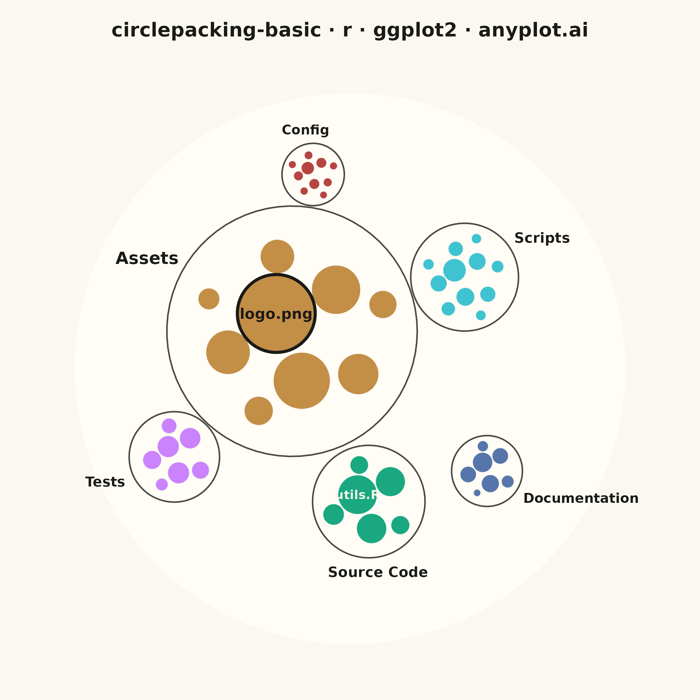
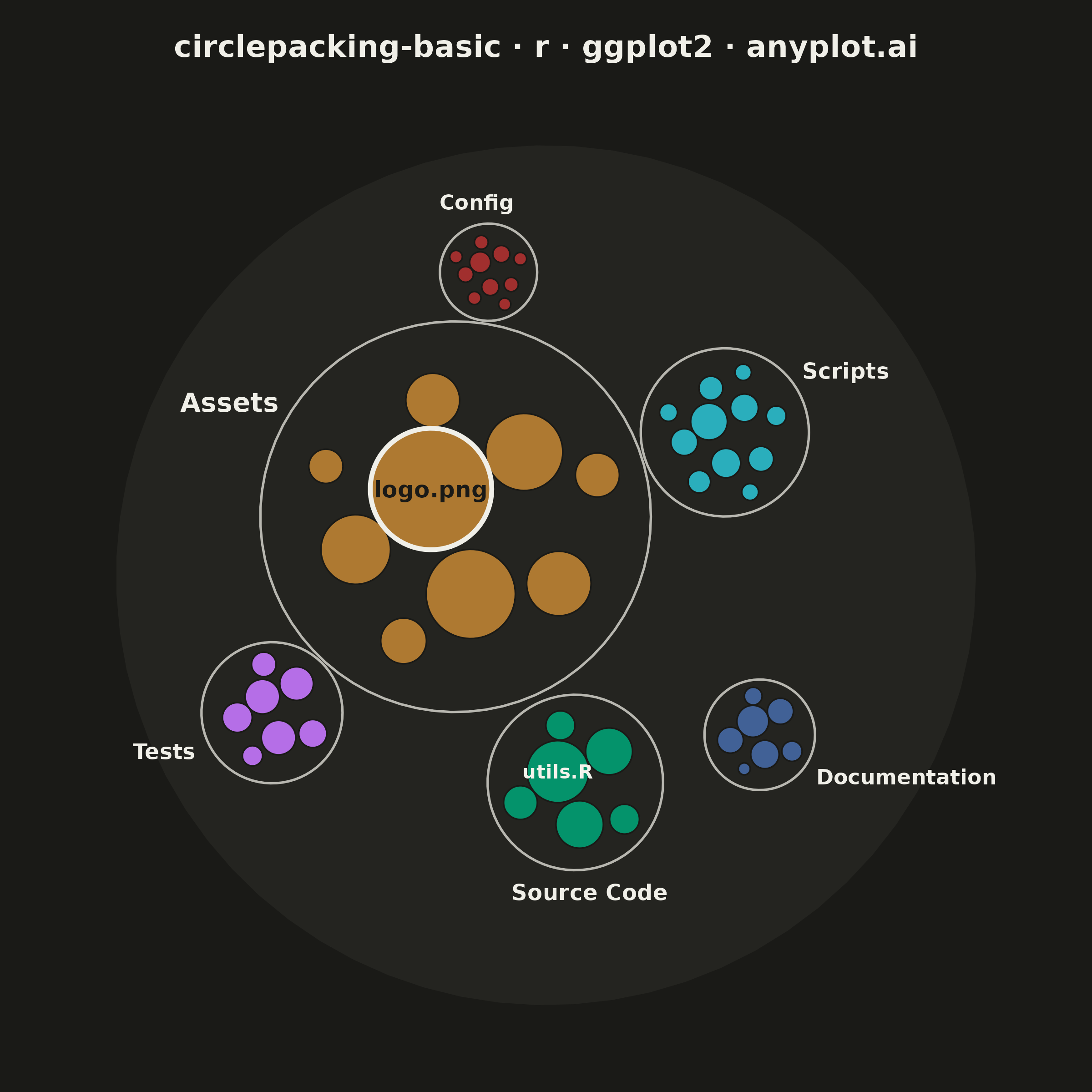
A circle packing chart displays hierarchical data as nested circles, where each circle contains smaller circles representing its children. Circle size is proportional to node value, and circles are packed efficiently without overlap. This visualization excels at revealing hierarchical structures while simultaneously showing quantitative relationships through area encoding.
#' anyplot.ai
#' circlepacking-basic: Circle Packing Chart
#' Library: ggplot2 3.5.1 | R 4.4.1
#' Quality: 90/100 | Created: 2026-09-02

library(ggplot2)
library(dplyr)
library(tibble)
library(ragg)

set.seed(42)

# --- Theme tokens -------------------------------------------------------
THEME       <- Sys.getenv("ANYPLOT_THEME", "light")
PAGE_BG     <- if (THEME == "light") "#FAF8F1" else "#1A1A17"
ELEVATED_BG <- if (THEME == "light") "#FFFDF6" else "#242420"
INK         <- if (THEME == "light") "#1A1A17" else "#F0EFE8"
INK_SOFT    <- if (THEME == "light") "#4A4A44" else "#B8B7B0"
IMPRINT_PALETTE <- c("#009E73", "#C475FD", "#4467A3", "#BD8233",
                     "#AE3030", "#2ABCCD", "#954477", "#99B314")

# --- Data: a repository's directory tree, sized by file weight (KB) -----
categories <- c("src", "tests", "docs", "assets", "config", "scripts")
category_labels <- c(
  src     = "Source Code",
  tests   = "Tests",
  docs    = "Documentation",
  assets  = "Assets",
  config  = "Config",
  scripts = "Scripts"
)
meanlog_by_cat <- c(src = 5.2, tests = 4.3, docs = 4.0, assets = 6.1, config = 3.0, scripts = 4.1)
sdlog_by_cat   <- c(src = 0.55, tests = 0.6, docs = 0.7, assets = 0.9, config = 0.5, scripts = 0.6)
file_pool <- list(
  src     = c("router", "auth", "database", "utils", "server", "api", "cache", "logger", "parser", "scheduler"),
  tests   = c("test_auth", "test_api", "test_database", "test_utils", "test_router", "test_cache"),
  docs    = c("readme", "architecture", "api-guide", "changelog", "contributing", "faq"),
  assets  = c("logo", "banner", "icon-set", "hero-image", "background", "favicon"),
  config  = c("app", "database", "logging", "ci", "docker", "eslint"),
  scripts = c("deploy", "build", "migrate", "seed", "backup", "release")
)
file_ext <- c(src = ".R", tests = ".R", docs = ".md", assets = ".png", config = ".yaml", scripts = ".sh")

leaves <- bind_rows(lapply(categories, function(category_name) {
  n_files <- sample(6:11, 1)
  names   <- sample(file_pool[[category_name]], n_files, replace = TRUE)
  tibble(
    category = category_name,
    id       = paste0(category_name, "_", sprintf("%02d", seq_len(n_files))),
    parent   = category_name,
    label    = paste0(names, file_ext[[category_name]]),
    value    = round(rlnorm(n_files, meanlog = meanlog_by_cat[[category_name]], sdlog = sdlog_by_cat[[category_name]]), 1)
  )
}))

# --- Circle packing: force-relaxation algorithm -------------------------
# Places circles of given radii tangent to their neighbours without
# overlap (spec: "Pack circles efficiently using force simulation"),
# then recenters the cluster on its own centroid.
pack_children <- function(radii, iterations = 500) {
  n <- length(radii)
  if (n == 1) {
    return(tibble(x = 0, y = 0, r = radii))
  }

  ord      <- order(radii, decreasing = TRUE)
  r_sorted <- radii[ord]
  padding  <- 0.03 * mean(r_sorted)

  golden_angle <- pi * (3 - sqrt(5))
  idx    <- seq_len(n)
  spread <- sum(r_sorted) * 0.5
  x <- spread * sqrt(idx / n) * cos(idx * golden_angle)
  y <- spread * sqrt(idx / n) * sin(idx * golden_angle)

  for (iter in seq_len(iterations)) {
    for (i in seq_len(n - 1)) {
      for (j in seq(i + 1, n)) {
        dx   <- x[j] - x[i]
        dy   <- y[j] - y[i]
        dist <- sqrt(dx^2 + dy^2)
        min_dist <- r_sorted[i] + r_sorted[j] + padding
        if (dist < min_dist) {
          if (dist < 1e-9) {
            dx <- runif(1, -1, 1); dy <- runif(1, -1, 1)
            dist <- sqrt(dx^2 + dy^2)
          }
          overlap <- (min_dist - dist) / 2
          ux <- dx / dist; uy <- dy / dist
          x[i] <- x[i] - ux * overlap; y[i] <- y[i] - uy * overlap
          x[j] <- x[j] + ux * overlap; y[j] <- y[j] + uy * overlap
        }
      }
    }
    x <- x - mean(x) * 0.02
    y <- y - mean(y) * 0.02
  }

  x <- x - mean(x)
  y <- y - mean(y)
  tibble(x = x[order(ord)], y = y[order(ord)], r = radii)
}

circle_points <- function(id, cx, cy, r, n = 72) {
  theta <- seq(0, 2 * pi, length.out = n)
  tibble(id = id, x = cx + r * cos(theta), y = cy + r * sin(theta))
}

# Level 1: pack leaf circles inside each category (area-accurate radius)
leaves_packed <- leaves %>%
  group_by(category) %>%
  group_modify(~ bind_cols(.x, pack_children(sqrt(.x$value / pi)))) %>%
  ungroup()

# Level 2: derive each category's outer radius from its packed children,
# then pack the categories inside the root with the same algorithm
category_stats <- leaves_packed %>%
  group_by(category) %>%
  summarise(enclose_r = max(sqrt(x^2 + y^2) + r), .groups = "drop") %>%
  mutate(
    draw_r = enclose_r * 1.15,
    label  = category_labels[category]
  ) %>%
  arrange(match(category, categories))

cat_positions <- pack_children(category_stats$draw_r)
category_stats$x_cat <- cat_positions$x
category_stats$y_cat <- cat_positions$y

root_r <- max(sqrt(category_stats$x_cat^2 + category_stats$y_cat^2) + category_stats$draw_r) * 1.14

leaves_final <- leaves_packed %>%
  left_join(category_stats %>% select(category, x_cat, y_cat), by = "category") %>%
  mutate(abs_x = x + x_cat, abs_y = y + y_cat)

# --- Polygons for rendering ----------------------------------------------
root_poly <- circle_points("root", 0, 0, root_r)

cat_polys <- bind_rows(Map(
  circle_points,
  id = category_stats$category, cx = category_stats$x_cat,
  cy = category_stats$y_cat, r = category_stats$draw_r
))

leaf_polys <- bind_rows(Map(
  circle_points,
  id = leaves_final$id, cx = leaves_final$abs_x,
  cy = leaves_final$abs_y, r = leaves_final$r
)) %>%
  left_join(leaves_final %>% select(id, category), by = "id")

cat_labels <- category_stats %>%
  mutate(
    dist_from_root = pmax(sqrt(x_cat^2 + y_cat^2), 1e-6),
    dir_x          = x_cat / dist_from_root,
    dir_y          = y_cat / dist_from_root,
    label_x        = x_cat + dir_x * (draw_r + root_r * 0.035),
    label_y        = y_cat + dir_y * (draw_r + root_r * 0.035),
    label_size     = 2.6 + 1.1 * (draw_r / max(draw_r)),
    # anchor the text edge (not its center) to the outward point, so the
    # whole label clears the circle boundary regardless of approach angle
    label_hjust = case_when(
      abs(dir_x) < abs(dir_y) ~ 0.5,
      dir_x >= 0               ~ 0,
      TRUE                     ~ 1
    ),
    label_vjust = case_when(
      abs(dir_y) <= abs(dir_x) ~ 0.5,
      dir_y >= 0                ~ 0,
      TRUE                      ~ 1
    )
  )

# --- Title (fontsize scales with title length) ---------------------------
plot_title <- "circlepacking-basic · r · ggplot2 · anyplot.ai"
title_n <- nchar(plot_title)
title_ratio <- if (title_n > 67) 67 / title_n else 1.0
title_fontsize <- max(8, round(12 * title_ratio))

fill_values <- setNames(IMPRINT_PALETTE[seq_along(categories)], categories)

# Text color per category chosen for contrast against that category's fill
# (data-tied, so — like the fill colors themselves — it does not flip with
# THEME).
pal_rgb        <- col2rgb(fill_values)
pal_luma       <- (0.299 * pal_rgb["red", ] + 0.587 * pal_rgb["green", ] + 0.114 * pal_rgb["blue", ]) / 255
leaf_label_ink <- ifelse(pal_luma < 0.5, "#F5F3EC", "#1A1A17")

# --- The largest leaf in each category, kept only for the 2 biggest ------
# categories, so every labeled circle is actually large enough to hold its
# text: a small category's own biggest leaf can still be too tiny to read.
leaf_top <- leaves_final %>%
  group_by(category) %>%
  slice_max(order_by = r, n = 1, with_ties = FALSE) %>%
  ungroup() %>%
  slice_max(order_by = r, n = 2, with_ties = FALSE) %>%
  mutate(
    label_size = pmin(3.2, pmax(1.8, 1.8 + 1.8 * (r / max(r)))),
    text_color = leaf_label_ink[category]
  )

focal_id   <- leaf_top$id[which.max(leaf_top$r)]
focal_ring <- leaf_polys %>% filter(id == focal_id)

# --- Plot ------------------------------------------------------------------
p <- ggplot() +
  geom_polygon(data = root_poly, aes(x, y), fill = ELEVATED_BG, color = NA) +
  geom_polygon(
    data = cat_polys, aes(x, y, group = id),
    fill = NA, color = INK_SOFT, linewidth = 0.45, alpha = 0.7
  ) +
  geom_polygon(
    data = leaf_polys, aes(x, y, group = id, fill = category),
    color = PAGE_BG, linewidth = 0.3, alpha = 0.9
  ) +
  geom_polygon(
    data = focal_ring, aes(x, y, group = id),
    fill = NA, color = INK, linewidth = 0.9
  ) +
  geom_text(
    data = cat_labels,
    aes(label_x, label_y, label = label, size = label_size, hjust = label_hjust, vjust = label_vjust),
    color = INK, fontface = "bold"
  ) +
  geom_text(
    data = leaf_top,
    aes(abs_x, abs_y, label = label, size = label_size, color = text_color),
    fontface = "bold"
  ) +
  scale_fill_manual(values = fill_values, guide = "none") +
  scale_color_identity() +
  scale_size_identity(guide = "none") +
  coord_fixed(
    xlim = c(-root_r * 1.12, root_r * 1.12),
    ylim = c(-root_r * 1.12, root_r * 1.12),
    expand = FALSE
  ) +
  labs(title = plot_title) +
  theme_void(base_size = 8) +
  theme(
    plot.background  = element_rect(fill = PAGE_BG, color = PAGE_BG),
    panel.background = element_rect(fill = PAGE_BG, color = NA),
    plot.title       = element_text(color = INK, size = title_fontsize, face = "bold", hjust = 0.5, margin = margin(b = 12)),
    plot.margin      = margin(14, 14, 14, 14)
  )

# --- Save --------------------------------------------------------------
ggsave(
  filename = sprintf("plot-%s.png", THEME),
  plot     = p,
  device   = ragg::agg_png,
  width    = 6,
  height   = 6,
  units    = "in",
  dpi      = 400
)
Runnable source as JSON, for any HTTP client: https://api.anyplot.ai/specs/circlepacking-basic/ggplot2/code. Any spec id and library id listed in llms-full.txt fit the same URL shape; every URL below is complete and callable.
{
  "spec_id": "circlepacking-basic",
  "language": "r",
  "library": "ggplot2",
  "page": "https://anyplot.ai/circlepacking-basic/r/ggplot2",
  "hub": "https://anyplot.ai/circlepacking-basic",
  "code_json": "https://api.anyplot.ai/specs/circlepacking-basic/ggplot2/code",
  "spec_json": "https://api.anyplot.ai/specs/circlepacking-basic",
  "render_light_png": "https://storage.googleapis.com/anyplot-images/plots/circlepacking-basic/r/ggplot2/plot-light.png",
  "render_dark_png": "https://storage.googleapis.com/anyplot-images/plots/circlepacking-basic/r/ggplot2/plot-dark.png",
  "quality_score": 90.0,
  "license": "MIT",
  "guide": "https://anyplot.ai/llms.txt"
}
Part of Circle Packing Chart on anyplot.ai.