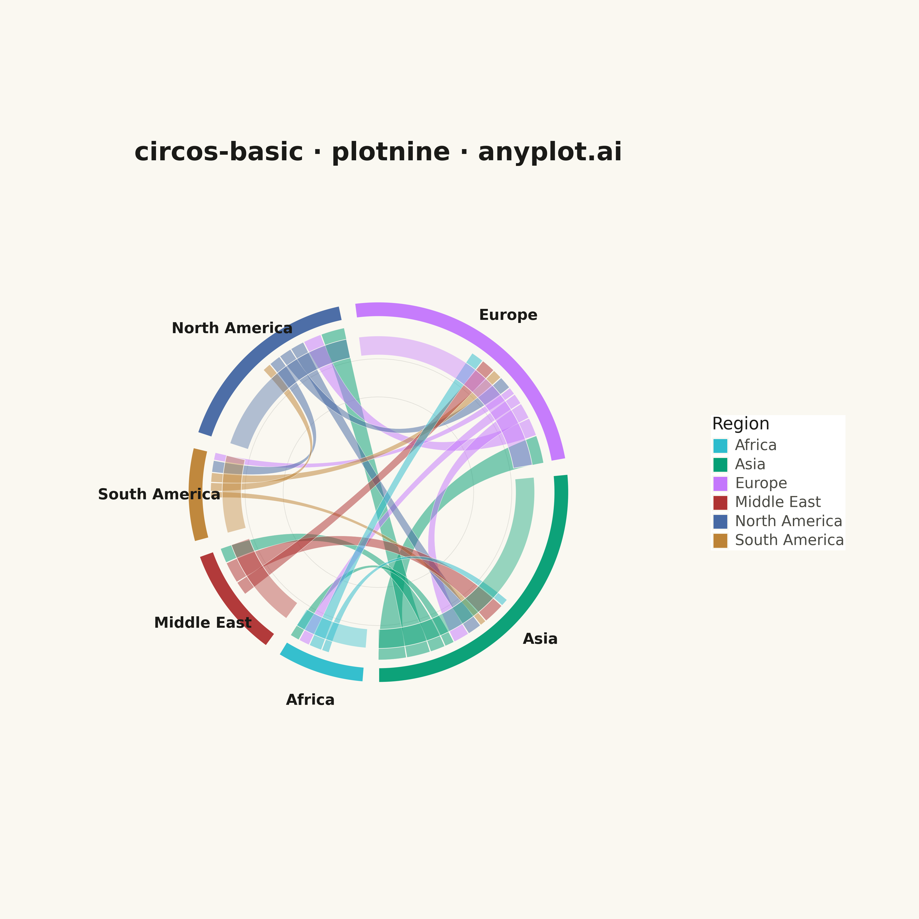
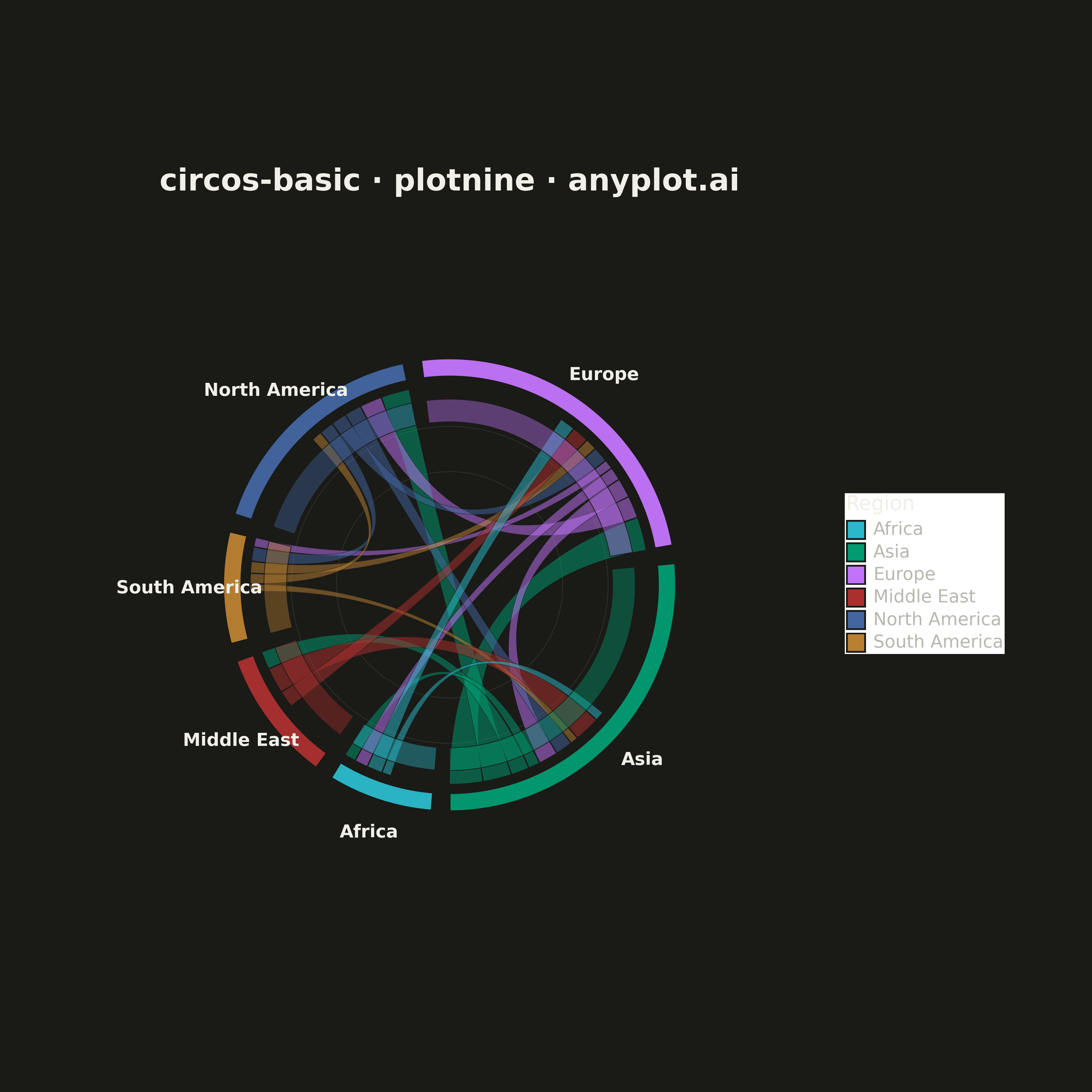
A Circos plot is a circular visualization that displays data on concentric tracks arranged around a circle, with ribbons or arcs connecting related segments across the circular layout. Originally designed for genomic data visualization, it excels at showing relationships between segments while simultaneously displaying multiple data attributes on different tracks. The circular arrangement makes efficient use of space and reveals patterns in complex relational data.
""" anyplot.ai
circos-basic: Circos Plot
Library: plotnine 0.15.4 | Python 3.13.13
Quality: 90/100 | Updated: 2026-05-15
"""

import os

import numpy as np
import pandas as pd
from plotnine import (
    aes,
    coord_fixed,
    element_blank,
    element_rect,
    element_text,
    geom_path,
    geom_polygon,
    geom_text,
    ggplot,
    labs,
    scale_fill_manual,
    scale_x_continuous,
    scale_y_continuous,
    theme,
)


# Theme tokens
THEME = os.getenv("ANYPLOT_THEME", "light")
PAGE_BG = "#FAF8F1" if THEME == "light" else "#1A1A17"
INK = "#1A1A17" if THEME == "light" else "#F0EFE8"
INK_SOFT = "#4A4A44" if THEME == "light" else "#B8B7B0"

# Okabe-Ito palette (first series is always #009E73)
IMPRINT = [
    "#009E73",  # bluish green (brand)
    "#C475FD",  # vermillion
    "#4467A3",  # blue
    "#BD8233",  # reddish purple
    "#AE3030",  # orange
    "#2ABCCD",  # sky blue
]

# Data - Trade flows between world regions
flows = [
    ("Asia", "Europe", 85),
    ("Asia", "North America", 72),
    ("Asia", "Middle East", 45),
    ("Asia", "Africa", 28),
    ("Europe", "North America", 55),
    ("Europe", "Asia", 48),
    ("Europe", "Africa", 32),
    ("Europe", "South America", 22),
    ("North America", "Asia", 42),
    ("North America", "Europe", 38),
    ("North America", "South America", 35),
    ("South America", "Europe", 28),
    ("South America", "North America", 25),
    ("South America", "Asia", 18),
    ("Middle East", "Asia", 65),
    ("Middle East", "Europe", 42),
    ("Africa", "Europe", 38),
    ("Africa", "Asia", 22),
]

# Unique segments
segments = list(dict.fromkeys([f[0] for f in flows] + [f[1] for f in flows]))

# Map segments to Okabe-Ito colors
colors = {seg: IMPRINT[i % len(IMPRINT)] for i, seg in enumerate(segments)}

# Calculate total flow for each segment
segment_totals = dict.fromkeys(segments, 0)
for src, tgt, val in flows:
    segment_totals[src] += val
    segment_totals[tgt] += val

total_flow = sum(segment_totals.values())

# Calculate arc positions
gap_angle = 0.08
total_gap = gap_angle * len(segments)
available_angle = 2 * np.pi - total_gap

segment_arcs = {}
current_angle = -np.pi / 2
for segment in segments:
    arc_size = (segment_totals[segment] / total_flow) * available_angle
    segment_arcs[segment] = {
        "start": current_angle,
        "end": current_angle + arc_size,
        "mid": current_angle + arc_size / 2,
    }
    current_angle += arc_size + gap_angle

# Radii for the circos plot
outer_radius = 1.0
inner_radius = 0.92
chord_radius = 0.88
track_outer = 0.82
track_inner = 0.72

# Build outer arc segments
arc_data = []
n_arc_points = 80
arc_id = 0
for segment in segments:
    arc = segment_arcs[segment]
    angles = np.linspace(arc["start"], arc["end"], n_arc_points)

    for angle in angles:
        arc_data.append(
            {
                "x": outer_radius * np.cos(angle),
                "y": outer_radius * np.sin(angle),
                "segment": segment,
                "arc_id": f"arc_{arc_id}",
            }
        )
    for angle in reversed(angles):
        arc_data.append(
            {
                "x": inner_radius * np.cos(angle),
                "y": inner_radius * np.sin(angle),
                "segment": segment,
                "arc_id": f"arc_{arc_id}",
            }
        )
    arc_id += 1

arc_df = pd.DataFrame(arc_data)

# Build inner data track
track_data = []
track_id = 0
for segment in segments:
    arc = segment_arcs[segment]
    angles = np.linspace(arc["start"], arc["end"], n_arc_points)

    for angle in angles:
        track_data.append(
            {
                "x": track_outer * np.cos(angle),
                "y": track_outer * np.sin(angle),
                "segment": segment,
                "track_id": f"track_{track_id}",
            }
        )
    for angle in reversed(angles):
        track_data.append(
            {
                "x": track_inner * np.cos(angle),
                "y": track_inner * np.sin(angle),
                "segment": segment,
                "track_id": f"track_{track_id}",
            }
        )
    track_id += 1

track_df = pd.DataFrame(track_data)

# Track segment offsets for chord placement
segment_offsets = {s: segment_arcs[s]["start"] for s in segments}

# Build ribbon/chord polygons
chord_data = []
chord_id = 0
n_bezier = 50

for src, tgt, val in flows:
    src_width = (val / total_flow) * available_angle * 0.5
    tgt_width = (val / total_flow) * available_angle * 0.5

    src_start = segment_offsets[src]
    src_end = src_start + src_width
    segment_offsets[src] = src_end + 0.005

    tgt_start = segment_offsets[tgt]
    tgt_end = tgt_start + tgt_width
    segment_offsets[tgt] = tgt_end + 0.005

    polygon_x = []
    polygon_y = []

    # Source arc
    src_angles = np.linspace(src_start, src_end, 15)
    for angle in src_angles:
        polygon_x.append(chord_radius * np.cos(angle))
        polygon_y.append(chord_radius * np.sin(angle))

    # Bezier from source to target
    src_end_x = chord_radius * np.cos(src_end)
    src_end_y = chord_radius * np.sin(src_end)
    tgt_start_x = chord_radius * np.cos(tgt_start)
    tgt_start_y = chord_radius * np.sin(tgt_start)

    for i in range(1, n_bezier):
        t = i / n_bezier
        x = (1 - t) ** 2 * src_end_x + 2 * (1 - t) * t * 0 + t**2 * tgt_start_x
        y = (1 - t) ** 2 * src_end_y + 2 * (1 - t) * t * 0 + t**2 * tgt_start_y
        polygon_x.append(x)
        polygon_y.append(y)

    # Target arc
    tgt_angles = np.linspace(tgt_start, tgt_end, 15)
    for angle in tgt_angles:
        polygon_x.append(chord_radius * np.cos(angle))
        polygon_y.append(chord_radius * np.sin(angle))

    # Bezier back from target to source
    tgt_end_x = chord_radius * np.cos(tgt_end)
    tgt_end_y = chord_radius * np.sin(tgt_end)
    src_start_x = chord_radius * np.cos(src_start)
    src_start_y = chord_radius * np.sin(src_start)

    for i in range(1, n_bezier):
        t = i / n_bezier
        x = (1 - t) ** 2 * tgt_end_x + 2 * (1 - t) * t * 0 + t**2 * src_start_x
        y = (1 - t) ** 2 * tgt_end_y + 2 * (1 - t) * t * 0 + t**2 * src_start_y
        polygon_x.append(x)
        polygon_y.append(y)

    for x, y in zip(polygon_x, polygon_y, strict=False):
        chord_data.append({"x": x, "y": y, "chord_id": f"chord_{chord_id}", "source": src, "target": tgt, "value": val})

    chord_id += 1

chord_df = pd.DataFrame(chord_data)

# Segment labels
label_data = []
label_radius = 1.15
for segment in segments:
    arc = segment_arcs[segment]
    mid_angle = arc["mid"]
    label_data.append(
        {
            "x": label_radius * np.cos(mid_angle),
            "y": label_radius * np.sin(mid_angle),
            "label": segment,
            "segment": segment,
        }
    )

label_df = pd.DataFrame(label_data)

# Circular gridlines
grid_rows = []
for radius in [0.5, 0.7]:
    grid_angles = np.linspace(0, 2 * np.pi, 100)
    for angle in grid_angles:
        grid_rows.append({"x": radius * np.cos(angle), "y": radius * np.sin(angle), "radius": radius})

grid_df = pd.DataFrame(grid_rows)

# Build the circos plot
plot = (
    ggplot()
    + geom_path(aes(x="x", y="y", group="radius"), data=grid_df, color=INK_SOFT, size=0.3, alpha=0.15)
    + geom_polygon(
        aes(x="x", y="y", group="chord_id", fill="source"), data=chord_df, alpha=0.5, color=PAGE_BG, size=0.15
    )
    + geom_polygon(
        aes(x="x", y="y", group="track_id", fill="segment"), data=track_df, alpha=0.4, color=PAGE_BG, size=0.3
    )
    + geom_polygon(aes(x="x", y="y", group="arc_id", fill="segment"), data=arc_df, alpha=0.95, color=PAGE_BG, size=0.8)
    + geom_text(aes(x="x", y="y", label="label"), data=label_df, size=14, color=INK, fontweight="bold")
    + scale_fill_manual(values=colors, name="Region")
    + coord_fixed(ratio=1)
    + scale_x_continuous(limits=(-1.6, 1.6), expand=(0, 0))
    + scale_y_continuous(limits=(-1.5, 1.6), expand=(0, 0))
    + labs(title="circos-basic · plotnine · anyplot.ai")
    + theme(
        figure_size=(12, 12),
        plot_background=element_rect(fill=PAGE_BG, color=PAGE_BG),
        panel_background=element_rect(fill=PAGE_BG, color=PAGE_BG),
        plot_title=element_text(size=24, ha="center", fontweight="bold", margin={"b": 20}, color=INK),
        plot_margin=0.08,
        axis_title=element_blank(),
        axis_text=element_blank(),
        axis_ticks=element_blank(),
        axis_line=element_blank(),
        panel_grid_major=element_blank(),
        panel_grid_minor=element_blank(),
        legend_title=element_text(size=16, color=INK),
        legend_text=element_text(size=14, color=INK_SOFT),
        legend_position="right",
    )
)

# Save
plot.save(f"plot-{THEME}.png", dpi=300)
Runnable source as JSON, for any HTTP client: https://api.anyplot.ai/specs/circos-basic/plotnine/code. Any spec id and library id listed in llms-full.txt fit the same URL shape; every URL below is complete and callable.
{
  "spec_id": "circos-basic",
  "language": "python",
  "library": "plotnine",
  "page": "https://anyplot.ai/circos-basic/python/plotnine",
  "hub": "https://anyplot.ai/circos-basic",
  "code_json": "https://api.anyplot.ai/specs/circos-basic/plotnine/code",
  "spec_json": "https://api.anyplot.ai/specs/circos-basic",
  "render_light_png": "https://storage.googleapis.com/anyplot-images/plots/circos-basic/python/plotnine/plot-light.png",
  "render_dark_png": "https://storage.googleapis.com/anyplot-images/plots/circos-basic/python/plotnine/plot-dark.png",
  "quality_score": 90.0,
  "license": "MIT",
  "guide": "https://anyplot.ai/llms.txt"
}
Part of Circos Plot on anyplot.ai.