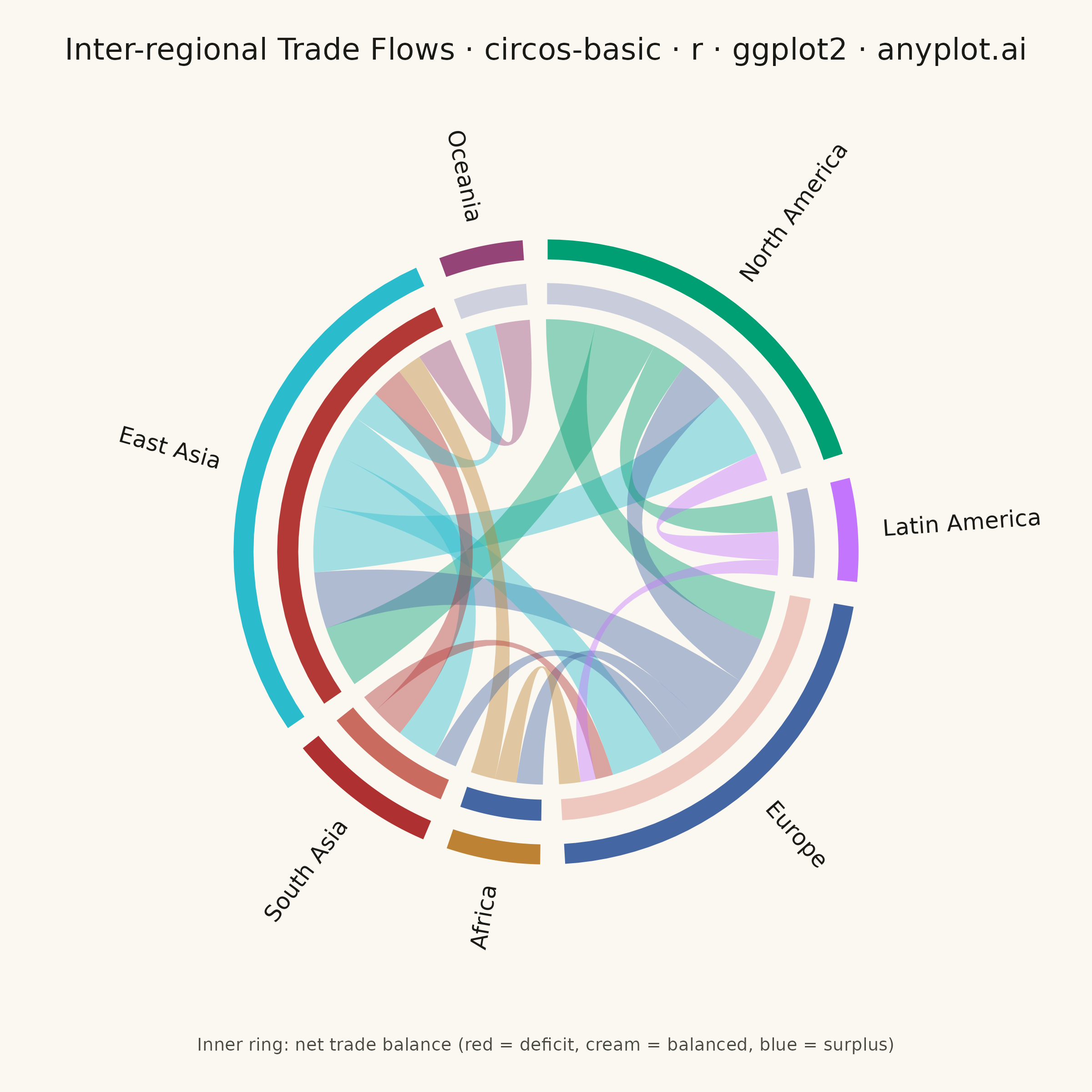
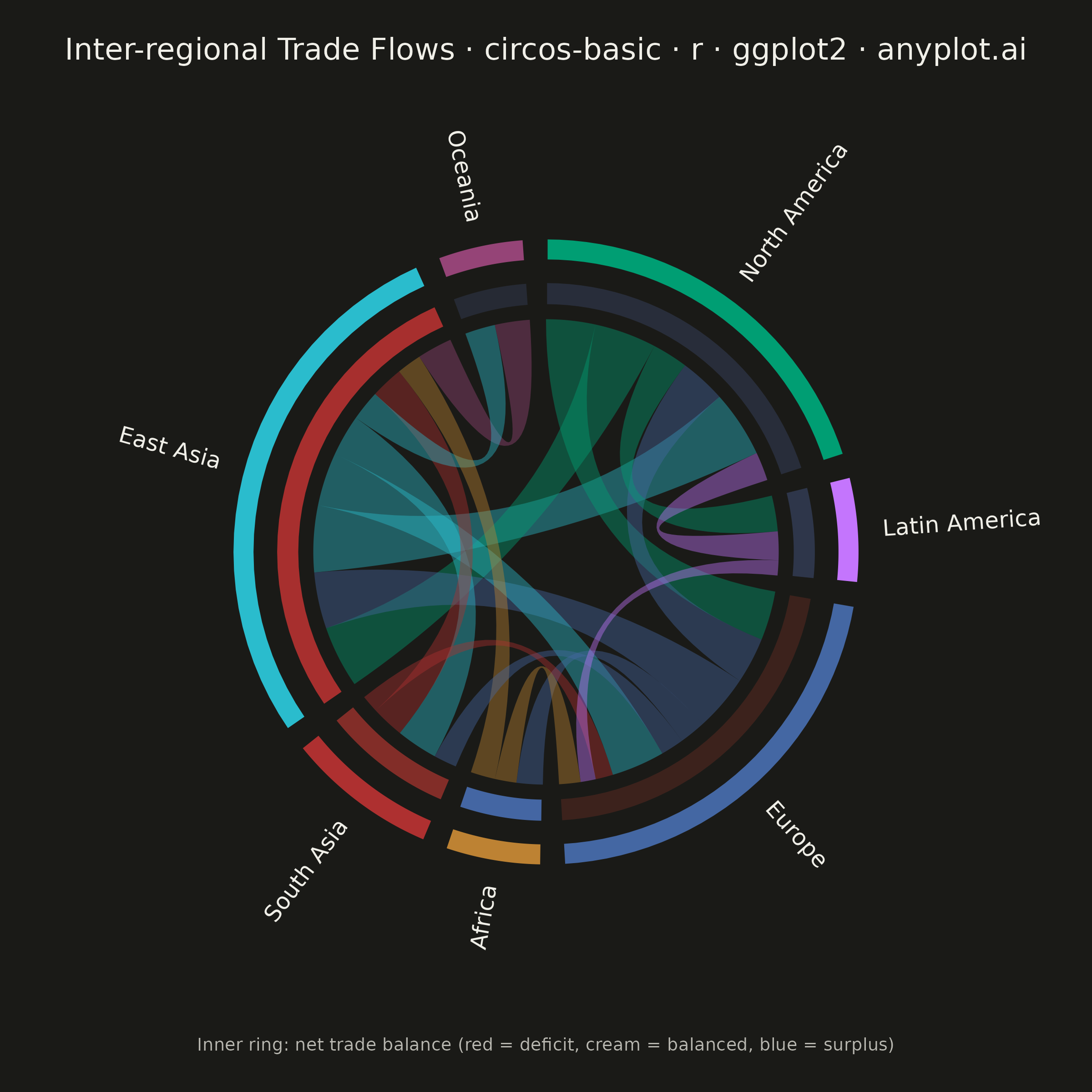
The same plot in 14 other libraries — Python: Altair, Bokeh, lets-plot, Matplotlib, Plotly, plotnine, Pygal, Seaborn; Julia: Makie.jl; JavaScript: Chart.js, D3.js, Apache ECharts, Highcharts, MUI X Charts. Compare all 15 side by side: Circos Plot in Python, R, Julia and JavaScript.
A Circos plot is a circular visualization that displays data on concentric tracks arranged around a circle, with ribbons or arcs connecting related segments across the circular layout. Originally designed for genomic data visualization, it excels at showing relationships between segments while simultaneously displaying multiple data attributes on different tracks. The circular arrangement makes efficient use of space and reveals patterns in complex relational data.
#' anyplot.ai
#' circos-basic: Circos Plot
#' Library: ggplot2 3.5.1 | R 4.4.1
#' Quality: 93/100 | Created: 2026-09-04

library(ggplot2)
library(dplyr)
library(tidyr)
library(ragg)

# --- Theme tokens ------------------------------------------------------------
THEME    <- Sys.getenv("ANYPLOT_THEME", "light")
PAGE_BG  <- if (THEME == "light") "#FAF8F1" else "#1A1A17"
INK      <- if (THEME == "light") "#1A1A17" else "#F0EFE8"
INK_SOFT <- if (THEME == "light") "#4A4A44" else "#B8B7B0"

IMPRINT_PALETTE <- c(
    "#009E73", "#C475FD", "#4467A3", "#BD8233",
    "#AE3030", "#2ABCCD", "#954477", "#99B314"
)

# --- Data: inter-regional trade flows (USD billions) -------------------------
segment_order <- c(
    "North America", "Latin America", "Europe",
    "Africa", "South Asia", "East Asia", "Oceania"
)

flows <- tibble::tribble(
    ~source,          ~target,          ~value,
    "North America",  "Europe",          62,
    "North America",  "East Asia",       78,
    "North America",  "Latin America",   45,
    "Europe",         "North America",   58,
    "Europe",         "East Asia",       71,
    "Europe",         "Africa",          33,
    "Europe",         "South Asia",      29,
    "East Asia",      "North America",   84,
    "East Asia",      "Europe",          67,
    "East Asia",      "South Asia",      52,
    "East Asia",      "Oceania",         38,
    "South Asia",     "East Asia",       41,
    "South Asia",     "Europe",          22,
    "Latin America",  "North America",   36,
    "Latin America",  "Europe",          19,
    "Africa",         "Europe",          27,
    "Africa",         "East Asia",       31,
    "Oceania",        "East Asia",       44
) %>%
    mutate(conn_id = row_number())

# --- Geometry helpers (circular layout has no native ggplot2 support) -------
deg2rad <- function(deg) deg * pi / 180

arc_path <- function(a0, a1, r, n = 30) {
    angles <- seq(a0, a1, length.out = n)
    data.frame(x = r * cos(deg2rad(angles)), y = r * sin(deg2rad(angles)))
}

bezier_path <- function(p0, p1, control = c(0, 0), n = 30) {
    t <- seq(0, 1, length.out = n)
    data.frame(
        x = (1 - t)^2 * p0[1] + 2 * (1 - t) * t * control[1] + t^2 * p1[1],
        y = (1 - t)^2 * p0[2] + 2 * (1 - t) * t * control[2] + t^2 * p1[2]
    )
}

polar_xy <- function(angle_deg, r) c(r * cos(deg2rad(angle_deg)), r * sin(deg2rad(angle_deg)))

# --- Segment sizing: arc length proportional to total flow touching it ------
gap_deg <- 4
n_seg   <- length(segment_order)

touches <- bind_rows(
    flows %>% transmute(segment = source, conn_id, value, role = "source"),
    flows %>% transmute(segment = target, conn_id, value, role = "target")
)

segment_totals <- touches %>%
    group_by(segment) %>%
    summarise(total = sum(value), .groups = "drop") %>%
    arrange(match(segment, segment_order)) %>%
    mutate(
        span = (360 - gap_deg * n_seg) * total / sum(total),
        color = IMPRINT_PALETTE[seq_len(n())]
    )

start_angle <- 90
angle_starts <- numeric(n_seg)
angle_ends   <- numeric(n_seg)
cur <- start_angle
for (i in seq_len(n_seg)) {
    angle_starts[i] <- cur
    angle_ends[i]   <- cur - segment_totals$span[i]
    cur <- angle_ends[i] - gap_deg
}
segment_totals$angle_start <- angle_starts
segment_totals$angle_end   <- angle_ends

# --- Trade balance per region (net exports − imports) → diverging track ----
balance <- flows %>%
    group_by(segment = source) %>%
    summarise(exports = sum(value), .groups = "drop") %>%
    full_join(
        flows %>% group_by(segment = target) %>% summarise(imports = sum(value), .groups = "drop"),
        by = "segment"
    ) %>%
    mutate(across(c(exports, imports), ~ replace_na(.x, 0)), net = exports - imports)

div_ramp <- grDevices::colorRamp(c("#AE3030", PAGE_BG, "#4467A3"), space = "Lab")
net_to_color <- function(net, max_abs) {
    t <- pmin(pmax((net / max_abs + 1) / 2, 0), 1)
    rgb_mat <- div_ramp(t)
    grDevices::rgb(rgb_mat[, 1], rgb_mat[, 2], rgb_mat[, 3], maxColorValue = 255)
}

segment_totals <- segment_totals %>%
    left_join(balance %>% select(segment, net), by = "segment") %>%
    mutate(track_color = net_to_color(net, max(abs(net))))

# --- Sub-arcs: divide each segment's span among its individual connections -
touches <- touches %>%
    left_join(segment_totals %>% select(segment, total, angle_start, angle_end), by = "segment") %>%
    arrange(segment, conn_id) %>%
    group_by(segment) %>%
    mutate(cum_before = cumsum(value) - value, cum_after = cumsum(value)) %>%
    ungroup() %>%
    mutate(
        seg_span = angle_start - angle_end,
        a0 = angle_start - seg_span * cum_before / total,
        a1 = angle_start - seg_span * cum_after / total
    )

ribbon_edges <- flows %>%
    left_join(
        touches %>% filter(role == "source") %>% transmute(conn_id, a0_s = a0, a1_s = a1),
        by = "conn_id"
    ) %>%
    left_join(
        touches %>% filter(role == "target") %>% transmute(conn_id, a0_t = a0, a1_t = a1),
        by = "conn_id"
    )

# --- Ribbon polygons: two arcs (at the sub-arc radius) joined by two Bezier
#     curves that sweep through the circle's center, the classic chord shape -
r_ribbon <- 1.00

ribbon_polygon <- function(row, r) {
    p_s1 <- polar_xy(row$a1_s, r)
    p_t0 <- polar_xy(row$a0_t, r)
    p_t1 <- polar_xy(row$a1_t, r)
    p_s0 <- polar_xy(row$a0_s, r)

    bind_rows(
        arc_path(row$a0_s, row$a1_s, r),
        bezier_path(p_s1, p_t0),
        arc_path(row$a0_t, row$a1_t, r),
        bezier_path(p_t1, p_s0)
    ) %>% mutate(conn_id = row$draw_order, source = row$source)
}

# Draw larger flows first and smaller ones last (on top) so thin connections
# stay traceable through the dense crossing zone near the center.
ribbon_edges <- ribbon_edges %>%
    arrange(desc(value)) %>%
    mutate(draw_order = row_number())

ribbons <- bind_rows(lapply(seq_len(nrow(ribbon_edges)), function(i) {
    ribbon_polygon(ribbon_edges[i, ], r_ribbon)
})) %>%
    left_join(segment_totals %>% select(segment, color), by = c("source" = "segment"))

# --- Track ring: constant-width band colored by net trade balance ----------
r_track_inner <- 1.06
r_track_outer <- 1.16

track_polys <- bind_rows(lapply(seq_len(nrow(segment_totals)), function(i) {
    seg <- segment_totals[i, ]
    bind_rows(
        arc_path(seg$angle_start, seg$angle_end, r_track_outer),
        arc_path(seg$angle_end, seg$angle_start, r_track_inner)
    ) %>% mutate(segment = seg$segment, color = seg$track_color)
}))

# --- Outer ring: one colored sector per segment -----------------------------
r_seg_inner <- 1.25
r_seg_outer <- 1.35

segment_polys <- bind_rows(lapply(seq_len(nrow(segment_totals)), function(i) {
    seg <- segment_totals[i, ]
    bind_rows(
        arc_path(seg$angle_start, seg$angle_end, r_seg_outer),
        arc_path(seg$angle_end, seg$angle_start, r_seg_inner)
    ) %>% mutate(segment = seg$segment, color = seg$color)
}))

# --- Segment labels, flipped on the circle's left half for legibility ------
segment_totals <- segment_totals %>%
    mutate(
        mid_angle   = (angle_start + angle_end) / 2,
        norm_angle  = ((mid_angle %% 360) + 360) %% 360,
        label_r     = r_seg_outer + 0.10,
        label_x     = label_r * cos(deg2rad(mid_angle)),
        label_y     = label_r * sin(deg2rad(mid_angle)),
        flipped     = norm_angle > 90 & norm_angle < 270,
        label_angle = ifelse(flipped, mid_angle + 180, mid_angle),
        label_hjust = ifelse(flipped, 1, 0)
    )

# --- Plot --------------------------------------------------------------------
title_text <- "Inter-regional Trade Flows · circos-basic · r · ggplot2 · anyplot.ai"
title_size <- max(8, round(12 * min(1, 67 / nchar(title_text))))

p <- ggplot() +
    geom_polygon(
        data = ribbons, aes(x, y, group = conn_id, fill = color),
        color = NA, alpha = 0.42
    ) +
    geom_polygon(
        data = track_polys, aes(x, y, group = segment, fill = color),
        color = PAGE_BG, linewidth = 0.4
    ) +
    geom_polygon(
        data = segment_polys, aes(x, y, group = segment, fill = color),
        color = PAGE_BG, linewidth = 0.6
    ) +
    geom_text(
        data = segment_totals,
        aes(x = label_x, y = label_y, label = segment, angle = label_angle, hjust = label_hjust),
        size = 3.2, color = INK, vjust = 0.5
    ) +
    scale_fill_identity() +
    coord_fixed(xlim = c(-1.8, 1.8), ylim = c(-1.8, 1.8), clip = "off") +
    labs(
        title   = title_text,
        caption = "Inner ring: net trade balance (red = deficit, cream = balanced, blue = surplus)"
    ) +
    theme_void(base_size = 8) +
    theme(
        plot.background  = element_rect(fill = PAGE_BG, color = PAGE_BG),
        panel.background = element_rect(fill = PAGE_BG, color = NA),
        plot.title       = element_text(color = INK, size = title_size, hjust = 0.5, margin = margin(b = 10)),
        plot.caption     = element_text(color = INK_SOFT, size = 7, hjust = 0.5, margin = margin(t = 10)),
        plot.margin      = margin(t = 15, r = 15, b = 15, l = 15)
    )

# --- Save (PNG, both themes) -------------------------------------------------
ggsave(
    filename = sprintf("plot-%s.png", THEME),
    plot     = p,
    device   = ragg::agg_png,
    width    = 6,
    height   = 6,
    units    = "in",
    dpi      = 400
)
Runnable source as JSON, for any HTTP client: https://api.anyplot.ai/specs/circos-basic/ggplot2/code. Any spec id and library id listed in llms-full.txt fit the same URL shape; every URL below is complete and callable.
{
  "spec_id": "circos-basic",
  "language": "r",
  "library": "ggplot2",
  "page": "https://anyplot.ai/circos-basic/r/ggplot2",
  "hub": "https://anyplot.ai/circos-basic",
  "code_json": "https://api.anyplot.ai/specs/circos-basic/ggplot2/code",
  "spec_json": "https://api.anyplot.ai/specs/circos-basic",
  "render_light_png": "https://storage.googleapis.com/anyplot-images/plots/circos-basic/r/ggplot2/plot-light.png",
  "render_dark_png": "https://storage.googleapis.com/anyplot-images/plots/circos-basic/r/ggplot2/plot-dark.png",
  "quality_score": 93.0,
  "license": "MIT",
  "guide": "https://anyplot.ai/llms.txt"
}
Part of Circos Plot on anyplot.ai.