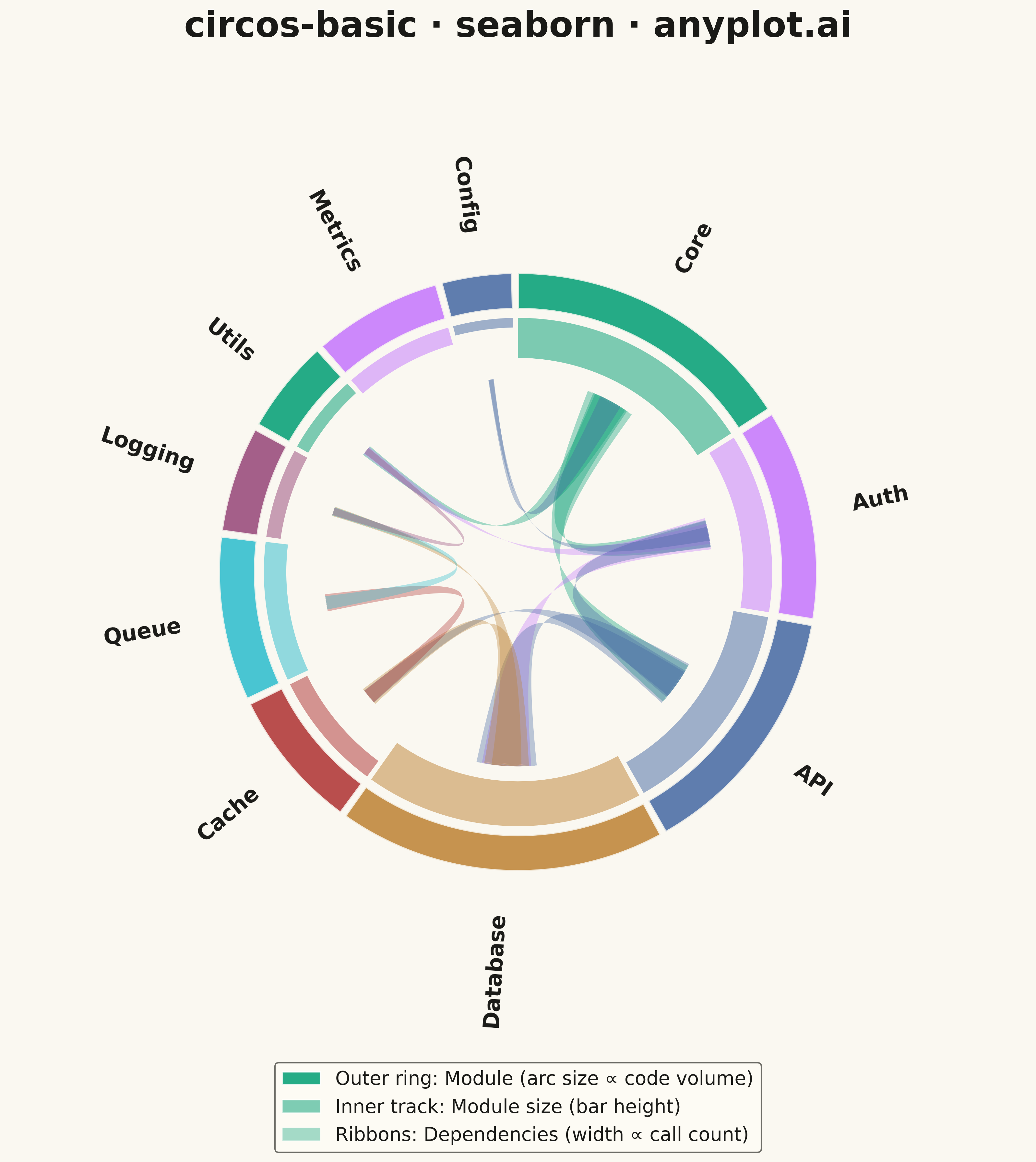
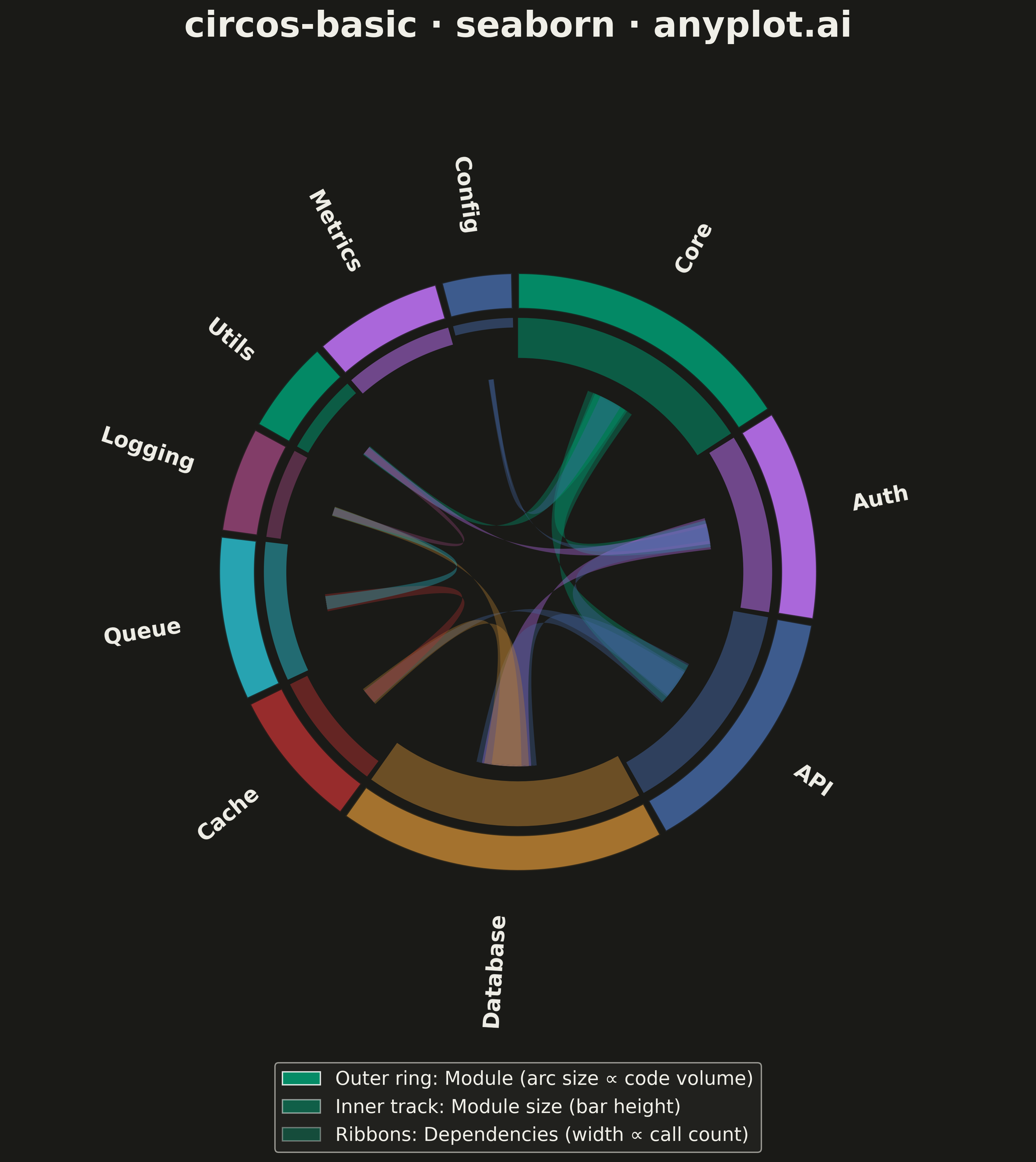
A Circos plot is a circular visualization that displays data on concentric tracks arranged around a circle, with ribbons or arcs connecting related segments across the circular layout. Originally designed for genomic data visualization, it excels at showing relationships between segments while simultaneously displaying multiple data attributes on different tracks. The circular arrangement makes efficient use of space and reveals patterns in complex relational data.
""" anyplot.ai
circos-basic: Circos Plot
Library: seaborn 0.13.2 | Python 3.13.13
Quality: 92/100 | Updated: 2026-05-15
"""

import os

import matplotlib.patches as mpatches
import matplotlib.pyplot as plt
import numpy as np
import seaborn as sns


# Theme tokens
THEME = os.getenv("ANYPLOT_THEME", "light")
PAGE_BG = "#FAF8F1" if THEME == "light" else "#1A1A17"
ELEVATED_BG = "#FFFDF6" if THEME == "light" else "#242420"
INK = "#1A1A17" if THEME == "light" else "#F0EFE8"
INK_SOFT = "#4A4A44" if THEME == "light" else "#B8B7B0"

# Okabe-Ito palette
IMPRINT = ["#009E73", "#C475FD", "#4467A3", "#BD8233", "#AE3030", "#2ABCCD", "#954477"]

# Set seaborn theme for consistent styling
sns.set_theme(
    style="white",
    rc={
        "figure.facecolor": PAGE_BG,
        "axes.facecolor": PAGE_BG,
        "axes.edgecolor": INK_SOFT,
        "axes.labelcolor": INK,
        "text.color": INK,
        "xtick.color": INK_SOFT,
        "ytick.color": INK_SOFT,
        "grid.color": INK,
        "grid.alpha": 0.10,
        "legend.facecolor": ELEVATED_BG,
        "legend.edgecolor": INK_SOFT,
    },
)

# Data: Software module dependencies (10 modules with inter-module calls)
np.random.seed(42)

# Define segments (modules) with their sizes (lines of code)
segments = ["Core", "Auth", "API", "Database", "Cache", "Queue", "Logging", "Utils", "Metrics", "Config"]
n_segments = len(segments)

# Segment sizes represent lines of code
segment_sizes = np.array([2500, 1800, 2200, 2800, 1200, 1400, 900, 800, 1100, 600])

# Create dependency connections (source module, target module, call count)
connections = [
    (0, 1, 45),  # Core -> Auth
    (0, 2, 65),  # Core -> API
    (0, 7, 38),  # Core -> Utils
    (1, 3, 55),  # Auth -> Database
    (1, 7, 28),  # Auth -> Utils
    (2, 1, 42),  # API -> Auth
    (2, 3, 72),  # API -> Database
    (2, 4, 35),  # API -> Cache
    (3, 4, 48),  # Database -> Cache
    (3, 6, 25),  # Database -> Logging
    (4, 5, 32),  # Cache -> Queue
    (5, 6, 20),  # Queue -> Logging
    (6, 7, 15),  # Logging -> Utils
    (9, 0, 18),  # Config -> Core
    (9, 1, 12),  # Config -> Auth
]

# Use Okabe-Ito palette, cycling through colors for segments
colors = [IMPRINT[i % len(IMPRINT)] for i in range(n_segments)]

# Create square figure for circular symmetry
fig, ax = plt.subplots(figsize=(12, 12), facecolor=PAGE_BG)
ax.set_facecolor(PAGE_BG)
ax.set_aspect("equal")

# Calculate segment positions (angles)
total_size = segment_sizes.sum()
gap_fraction = 0.02
total_gap = gap_fraction * n_segments
available_angle = 2 * np.pi * (1 - total_gap / (2 * np.pi))

angles = []
current_angle = np.pi / 2

for size in segment_sizes:
    segment_angle = (size / total_size) * available_angle
    start_angle = current_angle
    end_angle = current_angle - segment_angle
    angles.append((start_angle, end_angle))
    current_angle = end_angle - gap_fraction

# Draw outer ring segments
outer_radius = 1.0
ring_width = 0.12

for i, (start, end) in enumerate(angles):
    theta = np.linspace(end, start, 50)
    inner = outer_radius - ring_width
    x_outer = outer_radius * np.cos(theta)
    y_outer = outer_radius * np.sin(theta)
    x_inner = inner * np.cos(theta[::-1])
    y_inner = inner * np.sin(theta[::-1])
    x = np.concatenate([x_outer, x_inner])
    y = np.concatenate([y_outer, y_inner])
    ax.fill(x, y, color=colors[i], alpha=0.85, edgecolor=PAGE_BG, linewidth=1.5)

    # Add segment label
    mid_angle = (start + end) / 2
    label_radius = outer_radius + 0.14
    label_x = label_radius * np.cos(mid_angle)
    label_y = label_radius * np.sin(mid_angle)
    rotation_deg = np.degrees(mid_angle)
    norm_angle = rotation_deg % 360
    if 90 < norm_angle < 270:
        rotation = rotation_deg + 180
        ha = "right"
    else:
        rotation = rotation_deg
        ha = "left"
    ax.text(
        label_x,
        label_y,
        segments[i],
        ha=ha,
        va="center",
        fontsize=16,
        fontweight="bold",
        rotation=rotation,
        rotation_mode="anchor",
        color=INK,
    )

# Draw inner data track (code volume as bar heights)
inner_track_outer = outer_radius - ring_width - 0.03
inner_track_inner = inner_track_outer - 0.15

for i, (start, end) in enumerate(angles):
    height_fraction = segment_sizes[i] / segment_sizes.max()
    track_height = (inner_track_outer - inner_track_inner) * height_fraction
    theta = np.linspace(end, start, 30)
    inner = inner_track_outer - track_height
    x_outer = inner_track_outer * np.cos(theta)
    y_outer = inner_track_outer * np.sin(theta)
    x_inner = inner * np.cos(theta[::-1])
    y_inner = inner * np.sin(theta[::-1])
    x = np.concatenate([x_outer, x_inner])
    y = np.concatenate([y_outer, y_inner])
    ax.fill(x, y, color=colors[i], alpha=0.5, edgecolor="none")

# Draw ribbons (connections between modules)
ribbon_radius = inner_track_inner - 0.05
max_value = max(c[2] for c in connections)
min_value = min(c[2] for c in connections)
ctrl_radius = ribbon_radius * 0.1
n_points = 50
t = np.linspace(0, 1, n_points)

for source, target, value in connections:
    # Width calculation: map values to 0.25-0.7 range for better distinction
    normalized_value = (value - min_value) / (max_value - min_value)
    width_fraction = 0.25 + normalized_value * 0.45

    start1, end1 = angles[source]
    start2, end2 = angles[target]
    seg1_span = (start1 - end1) * width_fraction * 0.4
    seg2_span = (start2 - end2) * width_fraction * 0.4
    mid1 = (start1 + end1) / 2
    mid2 = (start2 + end2) / 2
    ribbon_start1 = mid1 + seg1_span / 2
    ribbon_end1 = mid1 - seg1_span / 2
    ribbon_start2 = mid2 + seg2_span / 2
    ribbon_end2 = mid2 - seg2_span / 2

    # First bezier curve
    p0 = np.array([ribbon_radius * np.cos(ribbon_start1), ribbon_radius * np.sin(ribbon_start1)])
    p3 = np.array([ribbon_radius * np.cos(ribbon_start2), ribbon_radius * np.sin(ribbon_start2)])
    p1 = ctrl_radius * np.array([np.cos(ribbon_start1), np.sin(ribbon_start1)])
    p2 = ctrl_radius * np.array([np.cos(ribbon_start2), np.sin(ribbon_start2)])
    curve1 = (
        (1 - t)[:, None] ** 3 * p0
        + 3 * (1 - t)[:, None] ** 2 * t[:, None] * p1
        + 3 * (1 - t)[:, None] * t[:, None] ** 2 * p2
        + t[:, None] ** 3 * p3
    )

    # Second bezier curve
    p0 = np.array([ribbon_radius * np.cos(ribbon_end1), ribbon_radius * np.sin(ribbon_end1)])
    p3 = np.array([ribbon_radius * np.cos(ribbon_end2), ribbon_radius * np.sin(ribbon_end2)])
    p1 = ctrl_radius * np.array([np.cos(ribbon_end1), np.sin(ribbon_end1)])
    p2 = ctrl_radius * np.array([np.cos(ribbon_end2), np.sin(ribbon_end2)])
    curve2 = (
        (1 - t)[:, None] ** 3 * p0
        + 3 * (1 - t)[:, None] ** 2 * t[:, None] * p1
        + 3 * (1 - t)[:, None] * t[:, None] ** 2 * p2
        + t[:, None] ** 3 * p3
    )

    # Arcs at source and target segments
    arc1_angles = np.linspace(ribbon_start1, ribbon_end1, 10)
    arc1 = ribbon_radius * np.column_stack([np.cos(arc1_angles), np.sin(arc1_angles)])
    arc2_angles = np.linspace(ribbon_end2, ribbon_start2, 10)
    arc2 = ribbon_radius * np.column_stack([np.cos(arc2_angles), np.sin(arc2_angles)])

    # Combine vertices and draw polygon with improved transparency
    vertices = np.vstack([arc1, curve1, arc2, curve2[::-1]])
    polygon = plt.Polygon(vertices, facecolor=colors[source], edgecolor="none", alpha=0.35, zorder=1)
    ax.add_patch(polygon)

# Configure axes
ax.set_xlim(-1.7, 1.7)
ax.set_ylim(-1.7, 1.7)
ax.axis("off")

# Title with correct format
ax.set_title("circos-basic · seaborn · anyplot.ai", fontsize=26, fontweight="bold", pad=20, color=INK)

# Add legend explaining the visualization
legend_elements = [
    mpatches.Patch(facecolor=IMPRINT[0], alpha=0.85, label="Outer ring: Module (arc size ∝ code volume)"),
    mpatches.Patch(facecolor=IMPRINT[0], alpha=0.5, label="Inner track: Module size (bar height)"),
    mpatches.Patch(facecolor=IMPRINT[0], alpha=0.35, label="Ribbons: Dependencies (width ∝ call count)"),
]
ax.legend(
    handles=legend_elements,
    loc="lower center",
    bbox_to_anchor=(0.5, -0.08),
    ncol=1,
    fontsize=14,
    frameon=True,
    facecolor=ELEVATED_BG,
    edgecolor=INK_SOFT,
)

plt.tight_layout()
plt.savefig(f"plot-{THEME}.png", dpi=300, bbox_inches="tight", facecolor=PAGE_BG)
Runnable source as JSON, for any HTTP client: https://api.anyplot.ai/specs/circos-basic/seaborn/code. Any spec id and library id listed in llms-full.txt fit the same URL shape; every URL below is complete and callable.
{
  "spec_id": "circos-basic",
  "language": "python",
  "library": "seaborn",
  "page": "https://anyplot.ai/circos-basic/python/seaborn",
  "hub": "https://anyplot.ai/circos-basic",
  "code_json": "https://api.anyplot.ai/specs/circos-basic/seaborn/code",
  "spec_json": "https://api.anyplot.ai/specs/circos-basic",
  "render_light_png": "https://storage.googleapis.com/anyplot-images/plots/circos-basic/python/seaborn/plot-light.png",
  "render_dark_png": "https://storage.googleapis.com/anyplot-images/plots/circos-basic/python/seaborn/plot-dark.png",
  "quality_score": 92.0,
  "license": "MIT",
  "guide": "https://anyplot.ai/llms.txt"
}
Part of Circos Plot on anyplot.ai.