The same plot in 14 other libraries — Python: Altair, Bokeh, lets-plot, Matplotlib, Plotly, plotnine, Pygal, Seaborn; Julia: Makie.jl; JavaScript: Chart.js, D3.js, Apache ECharts, Highcharts, MUI X Charts. Compare all 15 side by side: Confusion Matrix Heatmap in Python, R, Julia and JavaScript.
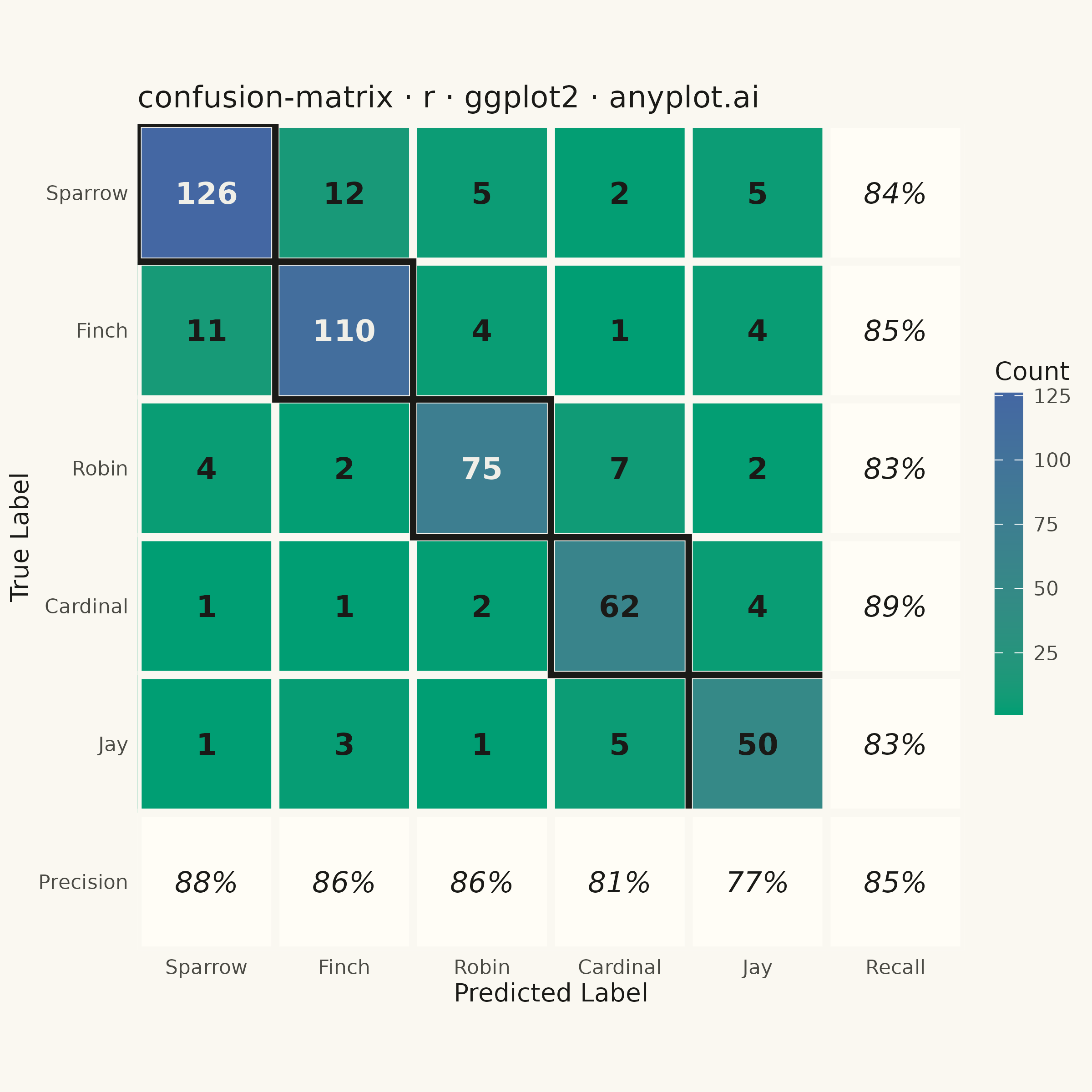
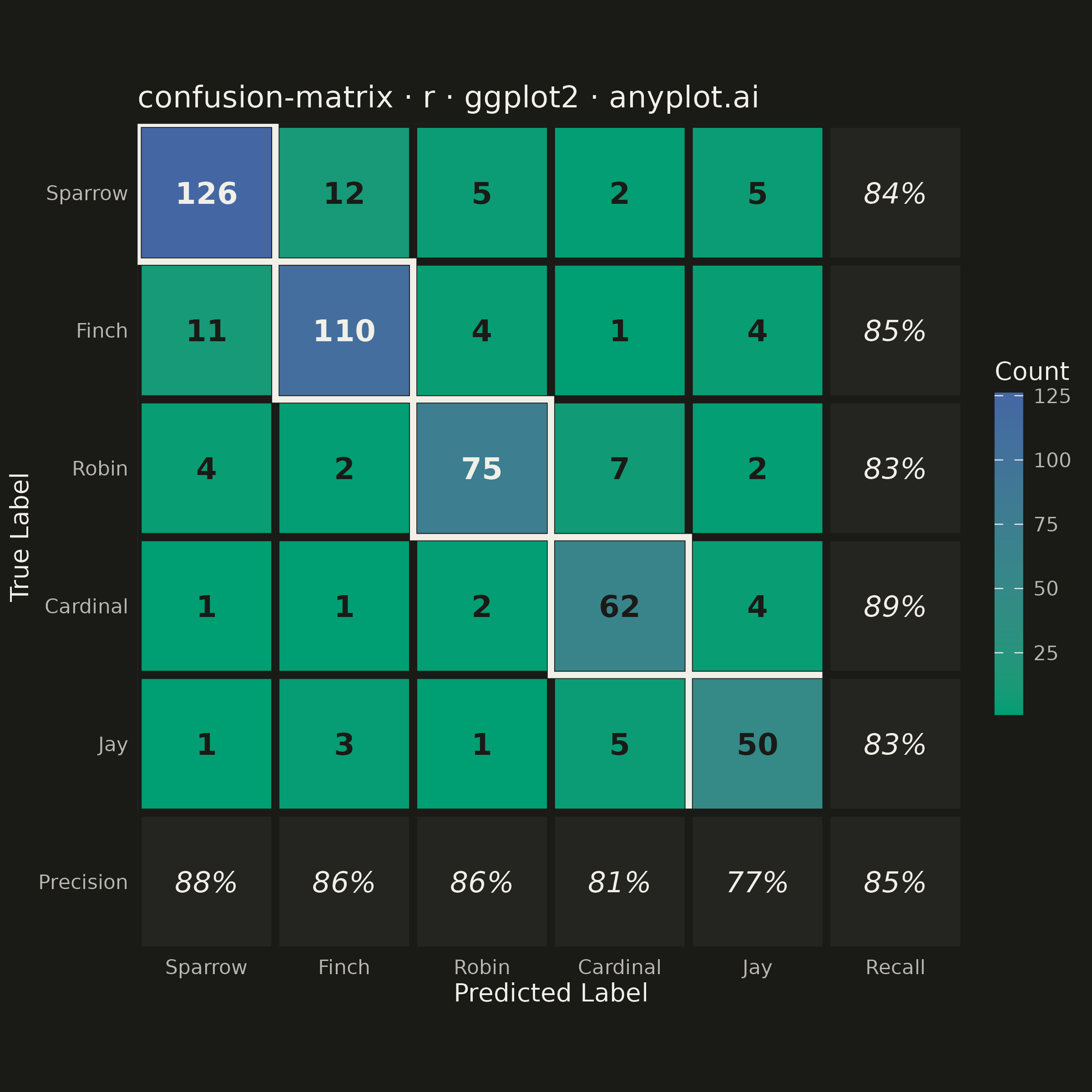
A specialized heatmap visualization for evaluating classification model performance, displaying the counts or proportions of predicted vs actual class labels. The confusion matrix reveals true positives, false positives, true negatives, and false negatives at a glance, making it essential for understanding model behavior, identifying class imbalances, and diagnosing specific misclassification patterns.
#' anyplot.ai
#' confusion-matrix: Confusion Matrix Heatmap
#' Library: ggplot2 3.5.1 | R 4.4.1
#' Quality: 92/100 | Created: 2026-09-04

library(ggplot2)
library(dplyr)
library(ragg)

set.seed(42)

# --- Theme tokens ------------------------------------------------------
THEME       <- Sys.getenv("ANYPLOT_THEME", "light")
PAGE_BG     <- if (THEME == "light") "#FAF8F1" else "#1A1A17"
ELEVATED_BG <- if (THEME == "light") "#FFFDF6" else "#242420"
INK         <- if (THEME == "light") "#1A1A17" else "#F0EFE8"
INK_SOFT    <- if (THEME == "light") "#4A4A44" else "#B8B7B0"
ANNOT_DARK  <- "#1A1A17"
ANNOT_LIGHT <- "#F0EFE8"

# --- Data: bird-species image classifier on a held-out test set --------
class_names <- c("Sparrow", "Finch", "Robin", "Cardinal", "Jay")
class_sizes <- c(150, 130, 90, 70, 60)  # class imbalance in the test set

confusion_probs <- matrix(c(
  0.88, 0.06, 0.02, 0.02, 0.02,
  0.08, 0.82, 0.04, 0.03, 0.03,
  0.03, 0.05, 0.85, 0.04, 0.03,
  0.02, 0.03, 0.05, 0.87, 0.03,
  0.03, 0.04, 0.03, 0.05, 0.85
), nrow = length(class_names), byrow = TRUE)

true_labels <- rep(class_names, times = class_sizes)
predicted_labels <- unlist(lapply(seq_along(class_names), function(i) {
  sample(class_names, size = class_sizes[i], replace = TRUE, prob = confusion_probs[i, ])
}))

cm <- as.data.frame(
  table(
    true_label      = factor(true_labels, levels = class_names),
    predicted_label = factor(predicted_labels, levels = class_names)
  )
)
names(cm)[names(cm) == "Freq"] <- "count"
cm <- cm %>%
  mutate(
    is_diagonal = true_label == predicted_label,
    label_color = if_else(count > max(count) * 0.5, ANNOT_LIGHT, ANNOT_DARK)
  )

# --- Normalization margins: recall (row), precision (column), accuracy ----
diag_cells   <- filter(cm, is_diagonal)
row_totals   <- cm %>% group_by(true_label) %>% summarise(total = sum(count), .groups = "drop")
col_totals   <- cm %>% group_by(predicted_label) %>% summarise(total = sum(count), .groups = "drop")
overall_acc  <- sum(diag_cells$count) / sum(cm$count)

recall_df <- diag_cells %>%
  left_join(row_totals, by = "true_label") %>%
  transmute(x = "Recall", y = as.character(true_label), label = sprintf("%.0f%%", 100 * count / total))

precision_df <- diag_cells %>%
  left_join(col_totals, by = "predicted_label") %>%
  transmute(x = as.character(predicted_label), y = "Precision", label = sprintf("%.0f%%", 100 * count / total))

corner_df <- data.frame(x = "Recall", y = "Precision", label = sprintf("%.0f%%", 100 * overall_acc))

margin_df <- bind_rows(recall_df, precision_df, corner_df)

x_levels <- c(class_names, "Recall")
y_levels <- c("Precision", rev(class_names))

# --- Plot ----------------------------------------------------------------
p <- ggplot(cm, aes(x = predicted_label, y = true_label, fill = count)) +
  geom_tile(color = PAGE_BG, linewidth = 1.5) +
  geom_tile(
    data = filter(cm, is_diagonal),
    fill = NA, color = INK, linewidth = 1.2
  ) +
  geom_text(aes(label = count, color = label_color), size = 4.2, fontface = "bold") +
  geom_tile(
    data = margin_df, aes(x = x, y = y),
    inherit.aes = FALSE, fill = ELEVATED_BG, color = PAGE_BG, linewidth = 1.5
  ) +
  geom_text(
    data = margin_df, aes(x = x, y = y, label = label),
    inherit.aes = FALSE, color = INK, size = 4.0, fontface = "italic"
  ) +
  scale_color_identity() +
  scale_fill_gradient(low = "#009E73", high = "#4467A3", name = "Count") +
  scale_x_discrete(limits = x_levels, expand = c(0, 0)) +
  scale_y_discrete(limits = y_levels, expand = c(0, 0)) +
  coord_fixed() +
  labs(
    x     = "Predicted Label",
    y     = "True Label",
    title = "confusion-matrix · r · ggplot2 · anyplot.ai"
  ) +
  theme_minimal(base_size = 8) +
  theme(
    plot.background    = element_rect(fill = PAGE_BG, color = PAGE_BG),
    panel.background   = element_rect(fill = PAGE_BG, color = NA),
    panel.grid         = element_blank(),
    axis.title         = element_text(color = INK, size = 10),
    axis.text          = element_text(color = INK_SOFT, size = 8),
    axis.ticks         = element_blank(),
    plot.title         = element_text(color = INK, size = 12),
    legend.background  = element_rect(fill = PAGE_BG, color = NA),
    legend.text        = element_text(color = INK_SOFT, size = 8),
    legend.title       = element_text(color = INK, size = 10),
    legend.key.height  = unit(0.9, "cm"),
    legend.key.width   = unit(0.4, "cm")
  )

# --- Save ------------------------------------------------------------------
ggsave(
  filename = sprintf("plot-%s.png", THEME),
  plot     = p,
  device   = ragg::agg_png,
  width    = 6,
  height   = 6,
  units    = "in",
  dpi      = 400
)
Runnable source as JSON, for any HTTP client: https://api.anyplot.ai/specs/confusion-matrix/ggplot2/code. Any spec id and library id listed in llms-full.txt fit the same URL shape; every URL below is complete and callable.
{
  "spec_id": "confusion-matrix",
  "language": "r",
  "library": "ggplot2",
  "page": "https://anyplot.ai/confusion-matrix/r/ggplot2",
  "hub": "https://anyplot.ai/confusion-matrix",
  "code_json": "https://api.anyplot.ai/specs/confusion-matrix/ggplot2/code",
  "spec_json": "https://api.anyplot.ai/specs/confusion-matrix",
  "render_light_png": "https://storage.googleapis.com/anyplot-images/plots/confusion-matrix/r/ggplot2/plot-light.png",
  "render_dark_png": "https://storage.googleapis.com/anyplot-images/plots/confusion-matrix/r/ggplot2/plot-dark.png",
  "quality_score": 92.0,
  "license": "MIT",
  "guide": "https://anyplot.ai/llms.txt"
}
Part of Confusion Matrix Heatmap on anyplot.ai.