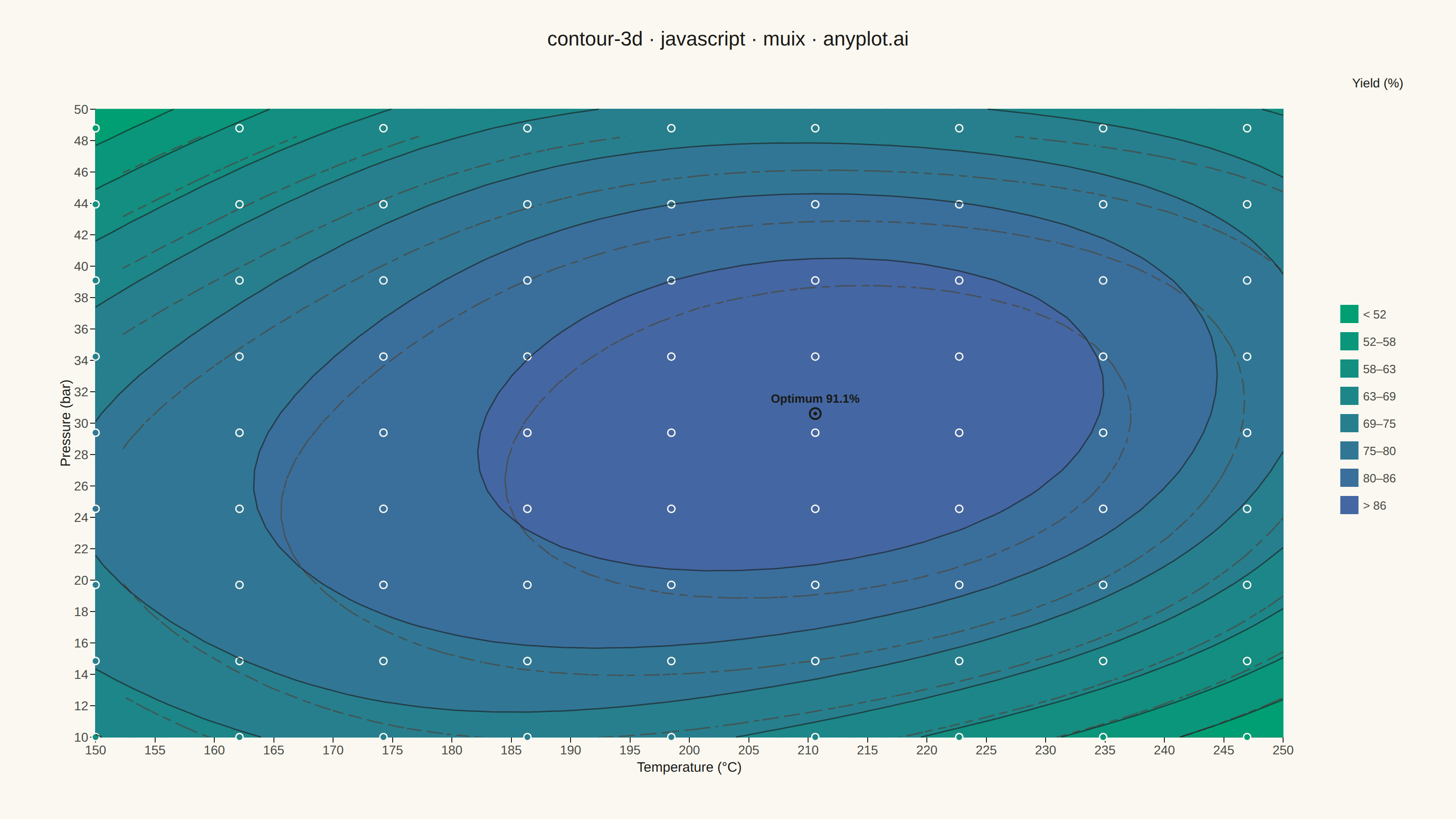
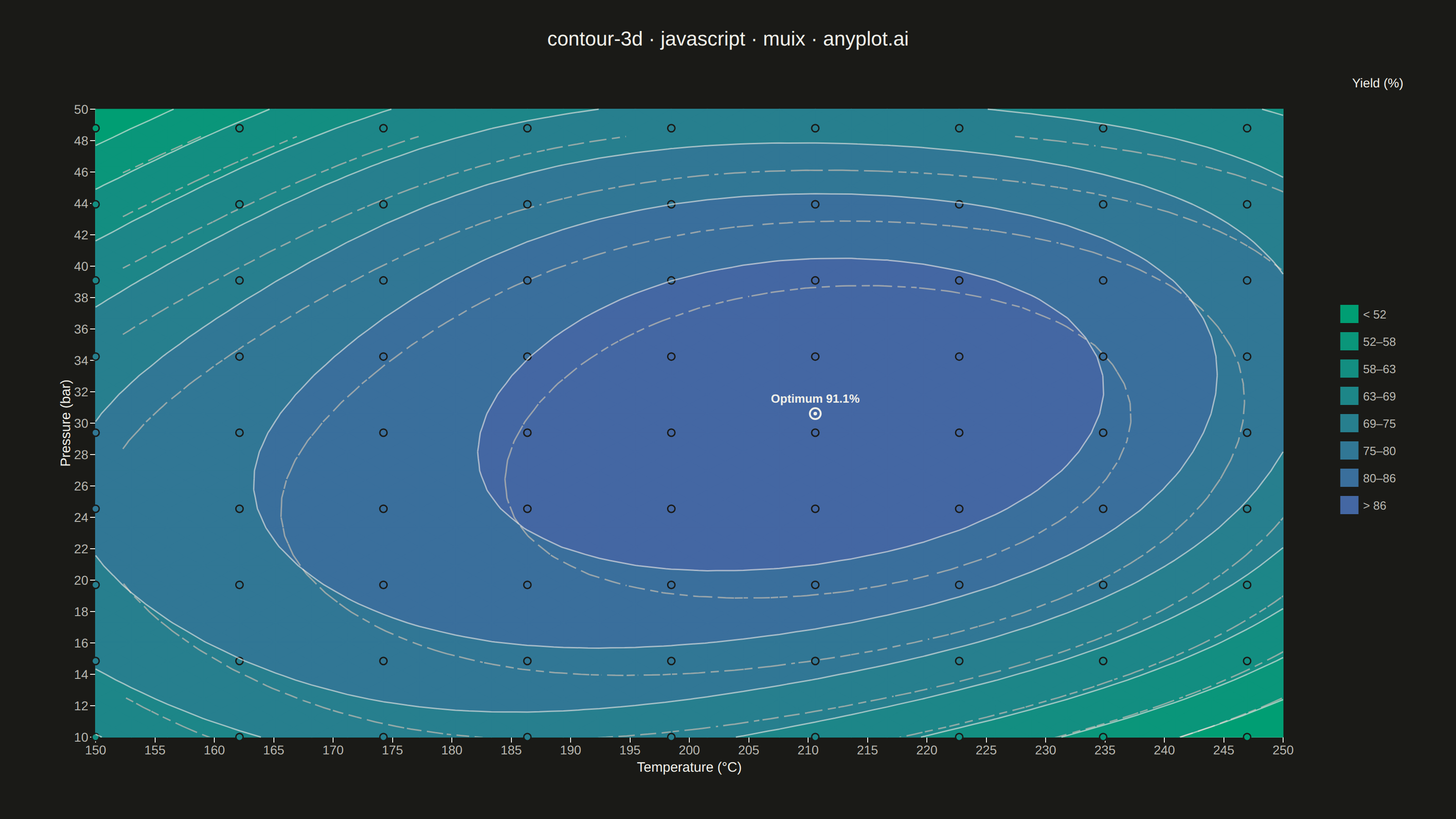
The same plot in 13 other libraries — JavaScript: Chart.js, D3.js, Apache ECharts, Highcharts; Python: Altair, Bokeh, lets-plot, Matplotlib, Plotly, Pygal, Seaborn; R: ggplot2; Julia: Makie.jl. Compare all 14 side by side: 3D Contour Plot in Python, R, Julia and JavaScript.
A 3D contour plot displays contour lines or filled contour bands on a three-dimensional surface, showing isolines of a function of two variables in 3D space. Unlike 2D contour plots that flatten the visualization, 3D contour plots preserve the surface geometry while highlighting level curves, making it easier to understand both the overall shape and specific value regions simultaneously. This visualization combines the spatial intuition of 3D surfaces with the precision of contour-based value identification.
// anyplot.ai
// contour-3d: 3D Contour Plot
// Library: muix 7.29.1 | JavaScript 22.23.2
// Quality: 82/100 | Created: 2026-09-10

// Community @mui/x-charts has no 3D/surface primitive. The elevation surface
// is built as a genuinely data-driven ScatterChart: every grid point is a
// real scatter datum (x, y, z) wired through a `zAxis` piecewise colorMap,
// and a custom `slots.scatter` renderer (same pattern used by
// heatmap-correlation) reads the library's own xScale/yScale/colorGetter to
// draw the elevation bands, contour isolines, and a sparse sample-point
// overlay whose marker colors come straight from that colorGetter -- not a
// second hand-rolled palette. The spec's "project contours onto the base
// plane" note is honored with a dashed, offset duplicate of the isolines
// painted on top of the bands (clipped to the axes, no edge bleed) -- a
// legible reference layer, not a near-duplicate of the solid ones.

import { ScatterChart } from "@mui/x-charts/ScatterChart";
import { PiecewiseColorLegend } from "@mui/x-charts/ChartsLegend";
import { ChartsText } from "@mui/x-charts/ChartsText";

const t = window.ANYPLOT_TOKENS;
const SIZE = window.ANYPLOT_SIZE;

// --- Grid: deterministic chemical-process yield response surface -----------
const GRID_N = 34;
const TEMP_MIN = 150, TEMP_MAX = 250;
const PRESSURE_MIN = 10, PRESSURE_MAX = 50;

const temps = Array.from(
  { length: GRID_N },
  (_, i) => TEMP_MIN + (i / (GRID_N - 1)) * (TEMP_MAX - TEMP_MIN),
);
const pressures = Array.from(
  { length: GRID_N },
  (_, j) => PRESSURE_MIN + (j / (GRID_N - 1)) * (PRESSURE_MAX - PRESSURE_MIN),
);

// Second-order response-surface model (classic RSM form: intercept + linear +
// quadratic + interaction terms) with a mild ripple so contour bands aren't
// perfectly elliptical -- gives the surface a visible saddle/critical-point
// region, matching the spec's "optimization landscape with critical points".
function yieldAt(temp, pressure) {
  const u = (temp - 200) / 50;
  const v = (pressure - 30) / 20;
  return 90 - 15 * u * u - 20 * v * v + 8 * u * v + 3 * Math.sin(3 * u) * Math.cos(2 * v);
}

// zGrid[j][i] = yield at (temps[i], pressures[j])
const zGrid = pressures.map((p) => temps.map((temp) => yieldAt(temp, p)));
const allZ = zGrid.flat();
const zMin = Math.min(...allZ);
const zMax = Math.max(...allZ);

// Locate the global optimum -- a real, computed "critical point" (spec:
// "optimization landscapes with critical points") to annotate on the surface.
let optimum = { i: 0, j: 0, z: -Infinity };
for (let j = 0; j < GRID_N; j += 1) {
  for (let i = 0; i < GRID_N; i += 1) {
    if (zGrid[j][i] > optimum.z) optimum = { i, j, z: zGrid[j][i] };
  }
}

// --- Real @mui/x-charts scatter series: every grid point is genuine data ---
// (feeds the ScatterChart's own zAxis colorMap / colorGetter pipeline below,
// not just a styling prop -- the library resolves per-point color from this.)
const points = [];
for (let j = 0; j < GRID_N; j += 1) {
  for (let i = 0; i < GRID_N; i += 1) {
    points.push({ id: `${i}-${j}`, x: temps[i], y: pressures[j], z: zGrid[j][i] });
  }
}

// --- Imprint sequential colormap (single-polarity data: t.seq = [green, blue]) -
function hexToRgb(hex) {
  const n = parseInt(hex.slice(1), 16);
  return [(n >> 16) & 255, (n >> 8) & 255, n & 255];
}
function lerpChannel(a, b, ratio) {
  return Math.round(a + (b - a) * ratio);
}
function imprintSeqInterpolator(stops) {
  const [lo, hi] = stops.map(hexToRgb);
  return (position) => {
    const [r, g, b] = [0, 1, 2].map((c) => lerpChannel(lo[c], hi[c], position));
    return `rgb(${r}, ${g}, ${b})`;
  };
}
const seqColor = imprintSeqInterpolator(t.seq);

const NUM_BANDS = 8;
const bandThresholds = Array.from(
  { length: NUM_BANDS - 1 },
  (_, k) => zMin + ((k + 1) / NUM_BANDS) * (zMax - zMin),
);
const bandColors = Array.from({ length: NUM_BANDS }, (_, k) => seqColor(k / (NUM_BANDS - 1)));

// --- Marching-triangles filled-contour geometry ------------------------------
// Each grid cell is split into 4 triangles around its centroid so every
// super-level-set boundary resolves without the marching-squares saddle
// ambiguity; painting bands low-to-high (painter's algorithm) then produces
// correct filled bands regardless of how many disjoint regions a level has.
function buildTriangles() {
  const tris = [];
  for (let j = 0; j < GRID_N - 1; j += 1) {
    for (let i = 0; i < GRID_N - 1; i += 1) {
      const sw = { x: temps[i], y: pressures[j], z: zGrid[j][i] };
      const se = { x: temps[i + 1], y: pressures[j], z: zGrid[j][i + 1] };
      const ne = { x: temps[i + 1], y: pressures[j + 1], z: zGrid[j + 1][i + 1] };
      const nw = { x: temps[i], y: pressures[j + 1], z: zGrid[j + 1][i] };
      const center = {
        x: (sw.x + se.x) / 2,
        y: (sw.y + nw.y) / 2,
        z: (sw.z + se.z + ne.z + nw.z) / 4,
      };
      tris.push([sw, se, center], [se, ne, center], [ne, nw, center], [nw, sw, center]);
    }
  }
  return tris;
}
const triangles = buildTriangles();

// Filled sub-polygon(s) of one triangle lying at/above `threshold`, plus the
// interpolated edge (if any) that traces the exact level curve through it.
function triangleFill(a, b, c, threshold) {
  const inA = a.z >= threshold, inB = b.z >= threshold, inC = c.z >= threshold;
  const nIn = (inA ? 1 : 0) + (inB ? 1 : 0) + (inC ? 1 : 0);
  const cross = (p, q) => {
    const ratio = (threshold - p.z) / (q.z - p.z);
    return { x: p.x + ratio * (q.x - p.x), y: p.y + ratio * (q.y - p.y) };
  };

  if (nIn === 0) return { polys: [], cut: null };
  if (nIn === 3) return { polys: [[a, b, c]], cut: null };

  if (nIn === 1) {
    if (inA) { const ab = cross(a, b), ca = cross(c, a); return { polys: [[a, ab, ca]], cut: [ab, ca] }; }
    if (inB) { const ab = cross(a, b), bc = cross(b, c); return { polys: [[b, bc, ab]], cut: [bc, ab] }; }
    const ca = cross(c, a), bc = cross(b, c);
    return { polys: [[c, ca, bc]], cut: [ca, bc] };
  }

  // nIn === 2 (exactly one vertex out)
  if (!inC) { const bc = cross(b, c), ca = cross(c, a); return { polys: [[a, b, bc, ca]], cut: [ca, bc] }; }
  if (!inA) { const ca = cross(c, a), ab = cross(a, b); return { polys: [[b, c, ca, ab]], cut: [ab, ca] }; }
  const ab = cross(a, b), bc = cross(b, c);
  return { polys: [[c, a, ab, bc]], cut: [bc, ab] };
}

// Bands k=1..NUM_BANDS-1 are computed from the triangulation; band k=0 is the
// full domain rect (everything is above zMin), painted first as the base layer.
const bandGeometry = [];
const isolineGeometry = [];
for (let k = 1; k < NUM_BANDS; k += 1) {
  const threshold = bandThresholds[k - 1];
  const polys = [];
  const segments = [];
  for (const tri of triangles) {
    const { polys: p, cut } = triangleFill(tri[0], tri[1], tri[2], threshold);
    if (p.length) polys.push(...p);
    if (cut) segments.push(cut);
  }
  bandGeometry.push(polys);
  isolineGeometry.push(segments);
}

// Sparse sample-point overlay (every 4th grid line -> ~9x9 points): a real
// subset of `points` above, drawn through the library's own `colorGetter` so
// the markers' colors come from the ScatterChart's zAxis colorMap, not a
// second hand-rolled color computation.
const SAMPLE_STEP = 4;
const sampleIndices = [];
for (let j = 0; j < GRID_N; j += SAMPLE_STEP) {
  for (let i = 0; i < GRID_N; i += SAMPLE_STEP) {
    sampleIndices.push(j * GRID_N + i);
  }
}

// --- Custom `slots.scatter` renderer: bands + isolines + sample points, all -
// mapped through the ScatterChart's own xScale/yScale, colored through its
// own colorGetter -- this IS the library's scatter slot, not a bolt-on layer.
const SHADOW_OFFSET = 30;

function ContourSurfaceRenderer(props) {
  const { series, xScale, yScale, colorGetter } = props;
  const toSVG = (x, y) => [xScale(x), yScale(y)];

  const polysToPath = (polys, dx = 0, dy = 0) =>
    polys
      .map((poly) => {
        const pts = poly.map((p) => toSVG(p.x, p.y));
        const head = `M ${(pts[0][0] + dx).toFixed(1)},${(pts[0][1] + dy).toFixed(1)}`;
        const tail = pts
          .slice(1)
          .map(([px, py]) => `L ${(px + dx).toFixed(1)},${(py + dy).toFixed(1)}`)
          .join(" ");
        return `${head} ${tail} Z`;
      })
      .join(" ");

  const segmentsToPath = (segments, dx = 0, dy = 0) =>
    segments
      .map(([p0, p1]) => {
        const [x0, y0] = toSVG(p0.x, p0.y);
        const [x1, y1] = toSVG(p1.x, p1.y);
        return `M ${(x0 + dx).toFixed(1)},${(y0 + dy).toFixed(1)} L ${(x1 + dx).toFixed(1)},${(y1 + dy).toFixed(1)}`;
      })
      .join(" ");

  const [rx0, ry0] = toSVG(TEMP_MIN, PRESSURE_MIN);
  const [rx1, ry1] = toSVG(TEMP_MAX, PRESSURE_MAX);
  const baseRectPath = (dx = 0, dy = 0) =>
    `M ${(rx0 + dx).toFixed(1)},${(ry0 + dy).toFixed(1)} L ${(rx1 + dx).toFixed(1)},${(ry0 + dy).toFixed(1)} L ${(rx1 + dx).toFixed(1)},${(ry1 + dy).toFixed(1)} L ${(rx0 + dx).toFixed(1)},${(ry1 + dy).toFixed(1)} Z`;

  const [ox, oy] = toSVG(temps[optimum.i], pressures[optimum.j]);

  // Clip the offset shadow layer to the plot's own rectangle so the
  // down-right offset never bleeds into the margin past the axes.
  const clipX = Math.min(rx0, rx1);
  const clipY = Math.min(ry0, ry1);
  const clipW = Math.abs(rx1 - rx0);
  const clipH = Math.abs(ry1 - ry0);

  return (
    <g>
      <clipPath id="contour-3d-plot-clip">
        <rect x={clipX} y={clipY} width={clipW} height={clipH} />
      </clipPath>

      {/* On-surface elevation bands, viewed from directly above */}
      <path d={baseRectPath()} fill={bandColors[0]} stroke={bandColors[0]} strokeWidth={0.75} />
      {bandGeometry.map((polys, idx) => (
        <path
          key={`band-${idx}`}
          d={polysToPath(polys)}
          fill={bandColors[idx + 1]}
          stroke={bandColors[idx + 1]}
          strokeWidth={0.75}
        />
      ))}

      {/* Contours projected onto the base plane: the fully opaque bands above
          tile the whole domain, so a filled shadow would never show through --
          instead this offset+dashed duplicate of the isolines is painted on
          TOP of the bands (still clipped to the axes, no edge bleed), reading
          as a clearly separate reference layer rather than a near-duplicate. */}
      <g clipPath="url(#contour-3d-plot-clip)" opacity={0.75}>
        {isolineGeometry.map((segments, idx) => (
          <path
            key={`shadow-iso-${idx}`}
            d={segmentsToPath(segments, SHADOW_OFFSET, SHADOW_OFFSET)}
            stroke={t.inkSoft}
            strokeWidth={1.6}
            strokeDasharray="9 6"
            fill="none"
          />
        ))}
      </g>

      {/* Sparse sample points -- real scatter data, colored via the chart's
          own colorGetter (zAxis piecewise colorMap), not a second palette. */}
      {sampleIndices.map((idx) => {
        const p = series.data[idx];
        const [px, py] = toSVG(p.x, p.y);
        return (
          <circle
            key={`sample-${p.id}`}
            cx={px}
            cy={py}
            r={4}
            fill={colorGetter ? colorGetter(idx) : t.ink}
            stroke={t.pageBg}
            strokeWidth={1.5}
          />
        );
      })}

      {/* Solid contour lines on the surface itself */}
      {isolineGeometry.map((segments, idx) => (
        <path
          key={`iso-${idx}`}
          d={segmentsToPath(segments)}
          stroke={t.ink}
          strokeOpacity={0.6}
          strokeWidth={1.5}
          fill="none"
        />
      ))}

      {/* Critical point: the computed global optimum, a genuine data callout */}
      <circle cx={ox} cy={oy} r={6} fill="none" stroke={t.ink} strokeWidth={2} />
      <circle cx={ox} cy={oy} r={2} fill={t.ink} />
      <text
        x={ox}
        y={oy - 12}
        textAnchor="middle"
        fontSize={13}
        fontWeight={600}
        fill={t.ink}
        fontFamily="inherit"
      >
        {`Optimum ${optimum.z.toFixed(1)}%`}
      </text>
    </g>
  );
}

// --- Chart (default-exported component — the harness mounts it) -------------
const TITLE = "contour-3d · javascript · muix · anyplot.ai";
const MARGIN = { top: 120, right: 190, bottom: 90, left: 105 };

// PiecewiseColorLegend anchors flush against the literal SVG width, ignoring
// MARGIN.right entirely (its `position: "right"` offset is `svgWidth -
// legendWidth`) -- so the whole right-side cluster (legend + its rotated axis
// title) is wrapped in this leftward shift to keep swatches off the true edge.
const RIGHT_EDGE_INSET = 46;

function bandLabel({ min, max }) {
  if (min === null) return `< ${Math.round(max)}`;
  if (max === null) return `> ${Math.round(min)}`;
  return `${Math.round(min)}–${Math.round(max)}`;
}

export default function Chart() {
  return (
    <ScatterChart
      width={SIZE.width}
      height={SIZE.height}
      margin={MARGIN}
      skipAnimation
      disableVoronoi
      series={[
        {
          id: "yield-surface",
          type: "scatter",
          data: points,
          label: "Yield (%)",
          zAxisId: "yield",
        },
      ]}
      xAxis={[
        {
          scaleType: "linear",
          min: TEMP_MIN,
          max: TEMP_MAX,
          label: "Temperature (°C)",
          labelStyle: { fontSize: 15, fill: t.ink },
          tickLabelStyle: { fontSize: 14, fill: t.inkSoft },
        },
      ]}
      yAxis={[
        {
          scaleType: "linear",
          min: PRESSURE_MIN,
          max: PRESSURE_MAX,
          label: "Pressure (bar)",
          labelStyle: { fontSize: 15, fill: t.ink },
          tickLabelStyle: { fontSize: 14, fill: t.inkSoft },
          slotProps: { axisLabel: { x: -58 } },
        },
      ]}
      zAxis={[
        {
          id: "yield",
          colorMap: {
            type: "piecewise",
            thresholds: bandThresholds,
            colors: bandColors,
          },
        },
      ]}
      slots={{ scatter: ContourSurfaceRenderer }}
      slotProps={{ legend: { hidden: true } }}
    >
      <g transform={`translate(${-RIGHT_EDGE_INSET}, 0)`}>
        <PiecewiseColorLegend
          axisId="yield"
          position={{ horizontal: "right", vertical: "middle" }}
          direction="column"
          labelStyle={{ fontSize: 13, fill: t.inkSoft }}
          labelFormatter={bandLabel}
        />
        <ChartsText
          text="Yield (%)"
          x={SIZE.width - 40}
          y={MARGIN.top - 24}
          style={{ fontSize: 14, fontWeight: 500, fill: t.ink, textAnchor: "middle" }}
        />
      </g>
      <ChartsText
        text={TITLE}
        x={SIZE.width / 2}
        y={50}
        style={{ fontSize: 22, fontWeight: 500, fill: t.ink, textAnchor: "middle" }}
      />
    </ScatterChart>
  );
}
Runnable source as JSON, for any HTTP client: https://api.anyplot.ai/specs/contour-3d/muix/code. Any spec id and library id listed in llms-full.txt fit the same URL shape; every URL below is complete and callable.
{
  "spec_id": "contour-3d",
  "language": "javascript",
  "library": "muix",
  "page": "https://anyplot.ai/contour-3d/javascript/muix",
  "hub": "https://anyplot.ai/contour-3d",
  "code_json": "https://api.anyplot.ai/specs/contour-3d/muix/code",
  "spec_json": "https://api.anyplot.ai/specs/contour-3d",
  "render_light_png": "https://storage.googleapis.com/anyplot-images/plots/contour-3d/javascript/muix/plot-light.png",
  "render_dark_png": "https://storage.googleapis.com/anyplot-images/plots/contour-3d/javascript/muix/plot-dark.png",
  "interactive_light_html": "https://storage.googleapis.com/anyplot-images/plots/contour-3d/javascript/muix/plot-light.html",
  "interactive_dark_html": "https://storage.googleapis.com/anyplot-images/plots/contour-3d/javascript/muix/plot-dark.html",
  "quality_score": 82.0,
  "license": "MIT",
  "guide": "https://anyplot.ai/llms.txt"
}
Part of 3D Contour Plot on anyplot.ai.