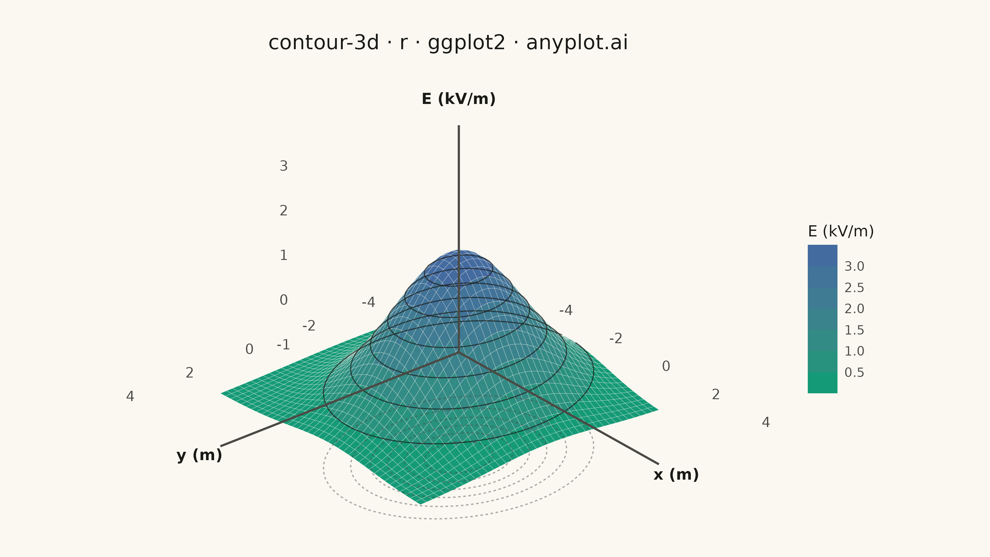
The same plot in 13 other libraries — Python: Altair, Bokeh, lets-plot, Matplotlib, Plotly, Pygal, Seaborn; Julia: Makie.jl; JavaScript: Chart.js, D3.js, Apache ECharts, Highcharts, MUI X Charts. Compare all 14 side by side: 3D Contour Plot in Python, R, Julia and JavaScript.
A 3D contour plot displays contour lines or filled contour bands on a three-dimensional surface, showing isolines of a function of two variables in 3D space. Unlike 2D contour plots that flatten the visualization, 3D contour plots preserve the surface geometry while highlighting level curves, making it easier to understand both the overall shape and specific value regions simultaneously. This visualization combines the spatial intuition of 3D surfaces with the precision of contour-based value identification.
#' anyplot.ai
#' contour-3d: 3D Contour Plot
#' Library: ggplot2 3.5.1 | R 4.4.1
#' Quality: 93/100 | Created: 2026-09-10

library(ggplot2)
library(dplyr)
library(ragg)

set.seed(42)

# --- Theme tokens -----------------------------------------------------------
THEME    <- Sys.getenv("ANYPLOT_THEME", "light")
PAGE_BG  <- if (THEME == "light") "#FAF8F1" else "#1A1A17"
INK      <- if (THEME == "light") "#1A1A17" else "#F0EFE8"
INK_SOFT <- if (THEME == "light") "#4A4A44" else "#B8B7B0"

# --- Camera: orthographic projection (elevation 28, azimuth 40) -------------
# ggplot2 has no 3D grammar, so the surface mesh and its contour isolines are
# projected to 2D screen coordinates ourselves (the same technique any static
# 3D renderer uses under the hood), then drawn with geom_polygon/geom_path.
elev <- 28 * pi / 180
azim <- 40 * pi / 180

view_dir <- c(cos(elev) * cos(azim), cos(elev) * sin(azim), sin(elev))
world_up <- c(0, 0, 1)
right_axis <- c(
  view_dir[2] * world_up[3] - view_dir[3] * world_up[2],
  view_dir[3] * world_up[1] - view_dir[1] * world_up[3],
  view_dir[1] * world_up[2] - view_dir[2] * world_up[1]
)
right_axis <- right_axis / sqrt(sum(right_axis^2))
up_axis <- c(
  right_axis[2] * view_dir[3] - right_axis[3] * view_dir[2],
  right_axis[3] * view_dir[1] - right_axis[1] * view_dir[3],
  right_axis[1] * view_dir[2] - right_axis[2] * view_dir[1]
)

Z_LIFT <- 1.3  # visual height exaggeration so the landscape reads clearly
project_x <- function(x, y, z) x * right_axis[1] + y * right_axis[2] + z * Z_LIFT * right_axis[3]
project_y <- function(x, y, z) x * up_axis[1]    + y * up_axis[2]    + z * Z_LIFT * up_axis[3]

# --- Data: electric field intensity around a point charge, 40x40 grid -------
# A single smooth peak keeps the equipotential isolines nested and legible in
# projection (a multi-peak landscape produces overlapping loops per level).
grid_n <- 40
x_vals <- seq(-4, 4, length.out = grid_n)
y_vals <- seq(-4, 4, length.out = grid_n)

field_intensity <- function(x1, x2) {
  3.4 * exp(-((x1 - 0.4)^2 / 5.0 + (x2 + 0.3)^2 / 7.2))
}
z_mat <- outer(x_vals, y_vals, field_intensity)

z_min <- min(z_mat)
z_max <- max(z_mat)
z_span <- z_max - z_min
floor_z <- z_min - 0.35 * z_span
ceil_z  <- z_max + 0.15 * z_span

x_min <- min(x_vals); x_max <- max(x_vals)
y_min <- min(y_vals); y_max <- max(y_vals)

# --- Bilinear interpolation so contour isolines get a surface height --------
interp_z <- function(x, y) {
  ix <- findInterval(x, x_vals, all.inside = TRUE)
  iy <- findInterval(y, y_vals, all.inside = TRUE)
  x0 <- x_vals[ix]; x1 <- x_vals[ix + 1]
  y0 <- y_vals[iy]; y1 <- y_vals[iy + 1]
  tx <- (x - x0) / (x1 - x0)
  ty <- (y - y0) / (y1 - y0)
  z00 <- z_mat[cbind(ix, iy)]
  z10 <- z_mat[cbind(ix + 1, iy)]
  z01 <- z_mat[cbind(ix, iy + 1)]
  z11 <- z_mat[cbind(ix + 1, iy + 1)]
  (z00 * (1 - tx) + z10 * tx) * (1 - ty) + (z01 * (1 - tx) + z11 * tx) * ty
}

# --- Surface as filled quads, painter's algorithm (far cells drawn first) ---
surface_quads <- vector("list", (grid_n - 1) * (grid_n - 1))
slot <- 0
for (i in seq_len(grid_n - 1)) {
  for (j in seq_len(grid_n - 1)) {
    slot <- slot + 1
    xs <- x_vals[c(i, i + 1, i + 1, i)]
    ys <- y_vals[c(j, j, j + 1, j + 1)]
    zs <- z_mat[cbind(c(i, i + 1, i + 1, i), c(j, j, j + 1, j + 1))]
    surface_quads[[slot]] <- data.frame(
      poly_id = slot,
      depth   = i + j,
      px      = project_x(xs, ys, zs),
      py      = project_y(xs, ys, zs),
      z_mid   = mean(zs)
    )
  }
}
surface_df <- bind_rows(surface_quads) |> arrange(desc(depth), poly_id)

# --- Contour isolines (equipotential lines): on the surface, and projected
# onto the base plane for reference ------------------------------------------
contour_levels <- pretty(c(z_min, z_max), n = 6)
contour_levels <- contour_levels[contour_levels > z_min & contour_levels < z_max]
raw_lines <- grDevices::contourLines(x_vals, y_vals, z_mat, levels = contour_levels)

surface_lines <- bind_rows(lapply(seq_along(raw_lines), function(k) {
  ln <- raw_lines[[k]]
  z_line <- interp_z(ln$x, ln$y)
  data.frame(line_id = k, px = project_x(ln$x, ln$y, z_line), py = project_y(ln$x, ln$y, z_line))
}))
base_lines <- bind_rows(lapply(seq_along(raw_lines), function(k) {
  ln <- raw_lines[[k]]
  data.frame(line_id = k, px = project_x(ln$x, ln$y, floor_z), py = project_y(ln$x, ln$y, floor_z))
}))

# --- Axis box: three edges meeting at the front-left-bottom corner ----------
axis_lines <- data.frame(
  x    = c(x_min, x_min, x_min),
  y    = c(y_min, y_min, y_min),
  z    = c(floor_z, floor_z, floor_z),
  xend = c(x_max, x_min, x_min),
  yend = c(y_min, y_max, y_min),
  zend = c(floor_z, floor_z, ceil_z)
)
axis_lines$px    <- project_x(axis_lines$x, axis_lines$y, axis_lines$z)
axis_lines$py    <- project_y(axis_lines$x, axis_lines$y, axis_lines$z)
axis_lines$pxend <- project_x(axis_lines$xend, axis_lines$yend, axis_lines$zend)
axis_lines$pyend <- project_y(axis_lines$xend, axis_lines$yend, axis_lines$zend)

x_breaks <- pretty(x_vals, n = 4); x_breaks <- x_breaks[x_breaks >= x_min & x_breaks <= x_max]
y_breaks <- pretty(y_vals, n = 4); y_breaks <- y_breaks[y_breaks >= y_min & y_breaks <= y_max]
z_breaks <- pretty(c(floor_z, ceil_z), n = 4); z_breaks <- z_breaks[z_breaks >= floor_z & z_breaks <= ceil_z]

# Large offsets keep the x-tick and y-tick label clusters from colliding near
# the shared corner — both grow away from the box along their own axis line.
# 0.45x the axis range clears the surface's projected silhouette even for the
# negative-side ticks nearest the tall part of the mesh (0.3x left "-4"/"-2"
# sitting on top of the surface after the Z_LIFT projection); the matching
# Z_TICK_OFFSET below is widened in step so the two label columns don't swap
# one collision (with the mesh) for another (with each other).
tick_gap <- 0.45 * (x_max - x_min)
ticks <- rbind(
  data.frame(x = x_breaks, y = y_min - tick_gap, z = floor_z, label = x_breaks),
  data.frame(x = x_min - tick_gap, y = y_breaks, z = floor_z, label = y_breaks)
)
ticks$px <- project_x(ticks$x, ticks$y, ticks$z)
ticks$py <- project_y(ticks$x, ticks$y, ticks$z)

# Z ticks sit on the vertical axis line itself; nudge the label text
# (not the axis line) sideways into the open gap left of the mesh. Widened
# alongside tick_gap above so the z-tick column stays clear of both the mesh
# and the (now farther-out) y-tick label column.
Z_TICK_OFFSET <- 4.5
z_ticks <- data.frame(x = x_min, y = y_min, z = z_breaks, label = z_breaks)
z_ticks$px <- project_x(z_ticks$x, z_ticks$y, z_ticks$z) - Z_TICK_OFFSET
z_ticks$py <- project_y(z_ticks$x, z_ticks$y, z_ticks$z)

axis_labels <- data.frame(
  x     = c(x_max + 0.7, x_min, x_min),
  y     = c(y_min, y_max + 0.7, y_min),
  z     = c(floor_z, floor_z, ceil_z + 0.6),
  label = c("x (m)", "y (m)", "E (kV/m)")
)
axis_labels$px <- project_x(axis_labels$x, axis_labels$y, axis_labels$z)
axis_labels$py <- project_y(axis_labels$x, axis_labels$y, axis_labels$z)

# --- Plot ---------------------------------------------------------------
p <- ggplot() +
  geom_polygon(
    data = surface_df, aes(px, py, group = poly_id, fill = z_mid),
    color = PAGE_BG, linewidth = 0.05
  ) +
  geom_path(
    data = base_lines, aes(px, py, group = line_id),
    color = INK_SOFT, linewidth = 0.35, alpha = 0.45, linetype = "22"
  ) +
  geom_path(
    data = surface_lines, aes(px, py, group = line_id),
    color = INK, linewidth = 0.3, alpha = 0.7
  ) +
  geom_segment(
    data = axis_lines, aes(x = px, y = py, xend = pxend, yend = pyend),
    color = INK_SOFT, linewidth = 0.6
  ) +
  geom_text(data = ticks, aes(px, py, label = label), color = INK_SOFT, size = 2.9) +
  geom_text(data = z_ticks, aes(px, py, label = label), color = INK_SOFT, size = 2.9) +
  geom_text(data = axis_labels, aes(px, py, label = label), color = INK, size = 3.2, fontface = "bold") +
  scale_fill_steps(
    low = "#009E73", high = "#4467A3", n.breaks = 7, name = "E (kV/m)"
  ) +
  labs(title = "contour-3d · r · ggplot2 · anyplot.ai") +
  coord_fixed(ratio = 1, clip = "off") +
  theme_void(base_size = 8) +
  theme(
    plot.background   = element_rect(fill = PAGE_BG, color = PAGE_BG),
    panel.background  = element_rect(fill = PAGE_BG, color = NA),
    plot.title        = element_text(color = INK, size = 12, hjust = 0.5, margin = margin(b = 14)),
    plot.margin       = margin(t = 20, r = 30, b = 10, l = 20),
    legend.background = element_rect(fill = PAGE_BG, color = NA),
    legend.text       = element_text(color = INK_SOFT, size = 7.5),
    legend.title      = element_text(color = INK, size = 9)
  )

# --- Save -----------------------------------------------------------------
ggsave(
  filename = sprintf("plot-%s.png", THEME),
  plot     = p,
  device   = ragg::agg_png,
  width    = 8,
  height   = 4.5,
  units    = "in",
  dpi      = 400
)
Runnable source as JSON, for any HTTP client: https://api.anyplot.ai/specs/contour-3d/ggplot2/code. Any spec id and library id listed in llms-full.txt fit the same URL shape; every URL below is complete and callable.
{
  "spec_id": "contour-3d",
  "language": "r",
  "library": "ggplot2",
  "page": "https://anyplot.ai/contour-3d/r/ggplot2",
  "hub": "https://anyplot.ai/contour-3d",
  "code_json": "https://api.anyplot.ai/specs/contour-3d/ggplot2/code",
  "spec_json": "https://api.anyplot.ai/specs/contour-3d",
  "render_light_png": "https://storage.googleapis.com/anyplot-images/plots/contour-3d/r/ggplot2/plot-light.png",
  "render_dark_png": "https://storage.googleapis.com/anyplot-images/plots/contour-3d/r/ggplot2/plot-dark.png",
  "quality_score": 93.0,
  "license": "MIT",
  "guide": "https://anyplot.ai/llms.txt"
}
Part of 3D Contour Plot on anyplot.ai.