The same plot in 13 other libraries — Python: Altair, Bokeh, lets-plot, Matplotlib, Plotly, Pygal, Seaborn; R: ggplot2; JavaScript: Chart.js, D3.js, Apache ECharts, Highcharts, MUI X Charts. Compare all 14 side by side: 3D Contour Plot in Python, R, Julia and JavaScript.
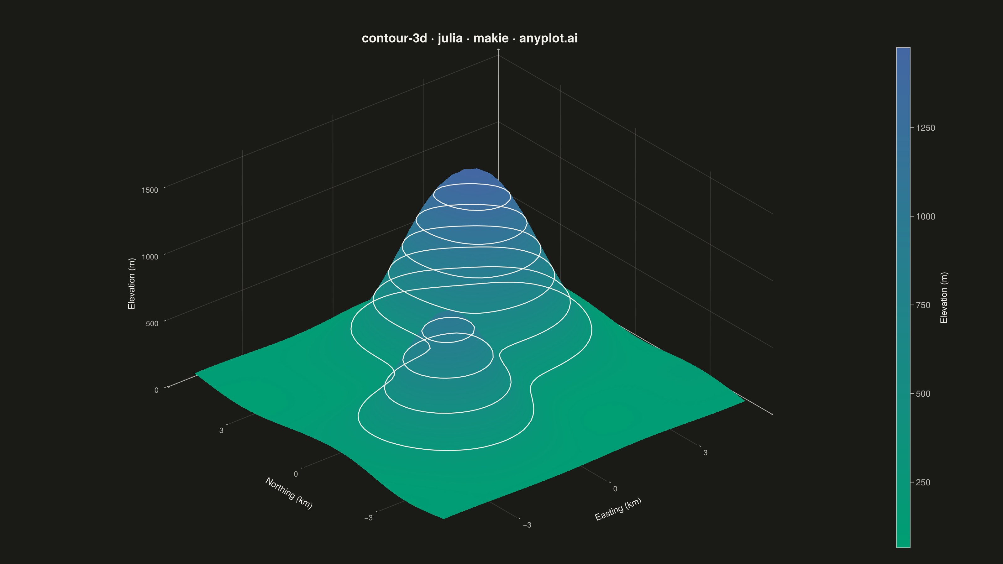
A 3D contour plot displays contour lines or filled contour bands on a three-dimensional surface, showing isolines of a function of two variables in 3D space. Unlike 2D contour plots that flatten the visualization, 3D contour plots preserve the surface geometry while highlighting level curves, making it easier to understand both the overall shape and specific value regions simultaneously. This visualization combines the spatial intuition of 3D surfaces with the precision of contour-based value identification.
# anyplot.ai
# contour-3d: 3D Contour Plot
# Library: makie 0.21.9 | Julia 1.11.9
# Quality: 81/100 | Created: 2026-09-10

using CairoMakie
using Colors

# --- Theme tokens -----------------------------------------------------------
const THEME    = get(ENV, "ANYPLOT_THEME", "light")
const PAGE_BG  = THEME == "light" ? colorant"#FAF8F1" : colorant"#1A1A17"
const INK      = THEME == "light" ? colorant"#1A1A17" : colorant"#F0EFE8"
const INK_SOFT = THEME == "light" ? colorant"#4A4A44" : colorant"#B8B7B0"

# Imprint sequential colormap — brand green to blue (default-style-guide.md
# "Continuous Data"). Elevation above sea level is single-polarity, so the
# diverging cmap is not appropriate here.
const IMPRINT_SEQ = cgrad([colorant"#009E73", colorant"#4467A3"])

# --- Data ---------------------------------------------------------------
# Synthetic mountain-range terrain survey: three peaks of different heights
# plus a gentle ripple for surface texture. Deterministic, no RNG needed.
easting = range(-5, 5, length=45)
northing = range(-5, 5, length=45)

elevation(e, n) =
    100 +
    1200 * exp(-((e - 1.5)^2) / 4 - ((n - 1.0)^2) / 3) +
    900 * exp(-((e + 2.0)^2) / 3 - ((n + 1.5)^2) / 2.5) +
    600 * exp(-((e - 0.5)^2) / 2 - ((n - 2.5)^2) / 2) +
    35 * sin(e) * cos(n)

z = [elevation(e, n) for e in easting, n in northing]

# --- Plot -----------------------------------------------------------------
title_str = "contour-3d · julia · makie · anyplot.ai"

fig = Figure(
    resolution      = (1600, 900),
    fontsize        = 14,
    backgroundcolor = PAGE_BG,
)

ax = Axis3(
    fig[1, 1];
    title              = title_str,
    titlesize          = 20,
    titlecolor         = INK,
    xlabel             = "Easting (km)",
    ylabel             = "Northing (km)",
    zlabel             = "Elevation (m)",
    xlabelsize         = 14,
    ylabelsize         = 14,
    zlabelsize         = 14,
    xlabelcolor        = INK,
    ylabelcolor        = INK,
    zlabelcolor        = INK,
    xticklabelsize     = 12,
    yticklabelsize     = 12,
    zticklabelsize     = 12,
    xticklabelcolor    = INK_SOFT,
    yticklabelcolor    = INK_SOFT,
    zticklabelcolor    = INK_SOFT,
    xtickcolor         = INK_SOFT,
    ytickcolor         = INK_SOFT,
    ztickcolor         = INK_SOFT,
    xspinecolor_1      = INK_SOFT,
    yspinecolor_1      = INK_SOFT,
    zspinecolor_1      = INK_SOFT,
    xspinecolor_2      = INK_SOFT,
    yspinecolor_2      = INK_SOFT,
    zspinecolor_2      = INK_SOFT,
    xspinecolor_3      = INK_SOFT,
    yspinecolor_3      = INK_SOFT,
    zspinecolor_3      = INK_SOFT,
    xgridcolor         = RGBAf(INK.r, INK.g, INK.b, 0.15),
    ygridcolor         = RGBAf(INK.r, INK.g, INK.b, 0.15),
    zgridcolor         = RGBAf(INK.r, INK.g, INK.b, 0.15),
    xypanelcolor       = PAGE_BG,
    xzpanelcolor       = PAGE_BG,
    yzpanelcolor       = PAGE_BG,
    backgroundcolor    = PAGE_BG,
    aspect             = (1, 1, 0.55),
    azimuth            = 1.28 * pi,
    elevation          = 0.16 * pi,
    protrusions        = (60, 60, 10, 60),
)

# Shaded surface preserving the terrain's 3D geometry
surf = surface!(ax, easting, northing, z; colormap = IMPRINT_SEQ, shading = NoShading)

# Isolines traced directly on the surface at their true elevation. Fewer,
# more widely spaced levels avoid two rings crowding into a near-solid disc
# on the shorter secondary peak.
contour3d!(ax, easting, northing, z; levels = 6, color = INK, linewidth = 1.5)

Colorbar(
    fig[1, 2], surf;
    label = "Elevation (m)", width = 22,
    labelcolor = INK, ticklabelcolor = INK_SOFT, tickcolor = INK_SOFT,
    leftspinecolor = INK_SOFT, rightspinecolor = INK_SOFT,
    topspinecolor = INK_SOFT, bottomspinecolor = INK_SOFT,
)

colsize!(fig.layout, 1, Relative(0.88))

# --- Save -------------------------------------------------------------------
save("plot-$(THEME).png", fig; px_per_unit = 2)
Runnable source as JSON, for any HTTP client: https://api.anyplot.ai/specs/contour-3d/makie/code. Any spec id and library id listed in llms-full.txt fit the same URL shape; every URL below is complete and callable.
{
  "spec_id": "contour-3d",
  "language": "julia",
  "library": "makie",
  "page": "https://anyplot.ai/contour-3d/julia/makie",
  "hub": "https://anyplot.ai/contour-3d",
  "code_json": "https://api.anyplot.ai/specs/contour-3d/makie/code",
  "spec_json": "https://api.anyplot.ai/specs/contour-3d",
  "render_light_png": "https://storage.googleapis.com/anyplot-images/plots/contour-3d/julia/makie/plot-light.png",
  "render_dark_png": "https://storage.googleapis.com/anyplot-images/plots/contour-3d/julia/makie/plot-dark.png",
  "quality_score": 81.0,
  "license": "MIT",
  "guide": "https://anyplot.ai/llms.txt"
}
Part of 3D Contour Plot on anyplot.ai.