The same plot in 14 other libraries — Python: Altair, Bokeh, lets-plot, Matplotlib, Plotly, plotnine, Pygal, Seaborn; R: ggplot2; JavaScript: Chart.js, D3.js, Apache ECharts, Highcharts, MUI X Charts. Compare all 15 side by side: Density Contour Plot in Python, R, Julia and JavaScript.
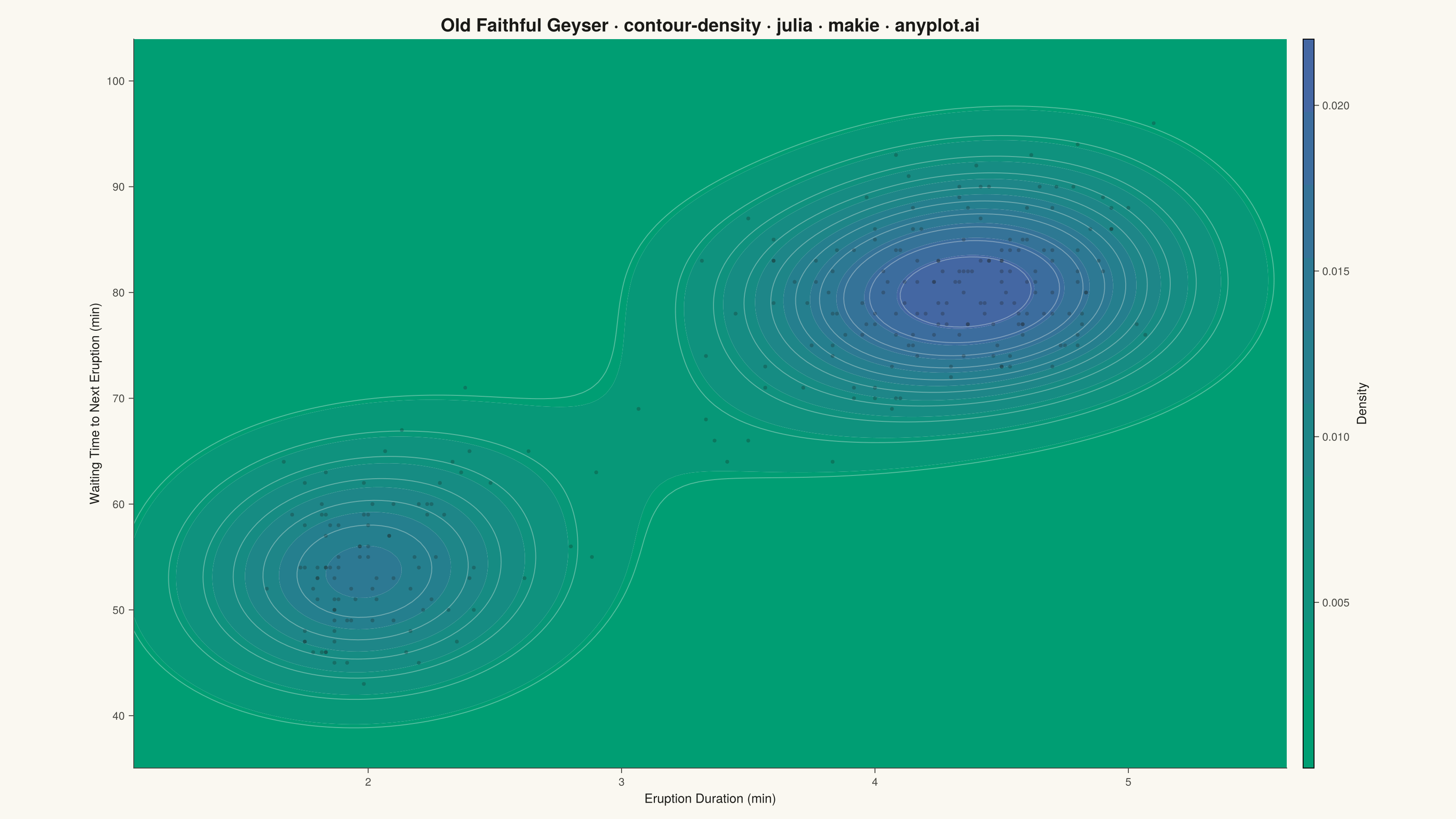
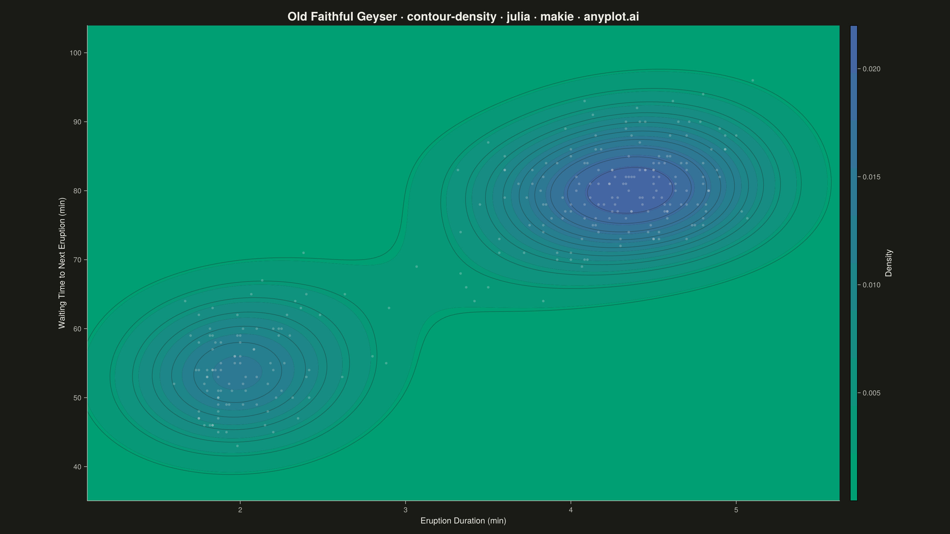
A density contour plot (also known as a 2D KDE contour plot) displays the concentration of points in a 2D scatter plot using contour lines. The contours connect points of equal density, revealing clusters, patterns, and the overall bivariate distribution shape.
# anyplot.ai
# contour-density: Density Contour Plot
# Library: makie 0.21.9 | Julia 1.11.9
# Quality: 89/100 | Created: 2026-09-04

using CairoMakie
using Colors
using RDatasets
using Statistics

# --- Theme tokens -----------------------------------------------------------
THEME    = get(ENV, "ANYPLOT_THEME", "light")
PAGE_BG  = THEME == "light" ? colorant"#FAF8F1" : colorant"#1A1A17"
INK      = THEME == "light" ? colorant"#1A1A17" : colorant"#F0EFE8"
INK_SOFT = THEME == "light" ? colorant"#4A4A44" : colorant"#B8B7B0"

# Imprint sequential colormap — density is single-polarity (concentration only)
ANYPLOT_SEQ = cgrad([colorant"#009E73", colorant"#4467A3"])

# Fixed (non-theme-flipping) ink for annotations placed on top of the density
# fill: the fill's colors are identical in both themes, and dark-on-fill
# measures ~5:1 contrast vs. ~3:1 for light-on-fill, so unlike the chrome,
# this text should NOT flip with THEME.
ANNOTATION_INK  = colorant"#1A1A17"
ANNOTATION_HALO = colorant"#FAF8F1"

# --- Data ---------------------------------------------------------------
# Old Faithful geyser: eruption duration vs. waiting time until next eruption.
# The classic bimodal bivariate dataset for demonstrating density contours.
faithful = RDatasets.dataset("datasets", "faithful")
duration = Float64.(faithful.Eruptions)
waiting  = Float64.(faithful.Waiting)
n        = length(duration)

# 2D Gaussian KDE evaluated on a regular grid, bandwidth via Silverman's rule.
pad_x  = 0.15 * (maximum(duration) - minimum(duration))
pad_y  = 0.15 * (maximum(waiting) - minimum(waiting))
xgrid  = range(minimum(duration) - pad_x, maximum(duration) + pad_x; length=150)
ygrid  = range(minimum(waiting) - pad_y, maximum(waiting) + pad_y; length=150)

bw_x = std(duration) * n^(-1 / 6)
bw_y = std(waiting) * n^(-1 / 6)

density = [
    sum(
        exp(-0.5 * (((xi - duration[k]) / bw_x)^2 + ((yi - waiting[k]) / bw_y)^2))
        for k in 1:n
    )
    for xi in xgrid, yi in ygrid
] ./ (n * 2π * bw_x * bw_y)

# --- Plot -----------------------------------------------------------------
fig = Figure(
    resolution      = (1600, 900),
    fontsize        = 14,
    backgroundcolor = PAGE_BG,
)

ax = Axis(
    fig[1, 1];
    title              = "Old Faithful Geyser · contour-density · julia · makie · anyplot.ai",
    titlesize          = 20,
    titlecolor         = INK,
    xlabel             = "Eruption Duration (min)",
    ylabel             = "Waiting Time to Next Eruption (min)",
    xlabelsize         = 14,
    ylabelsize         = 14,
    xlabelcolor        = INK,
    ylabelcolor        = INK,
    xticklabelsize     = 12,
    yticklabelsize     = 12,
    xticklabelcolor    = INK_SOFT,
    yticklabelcolor    = INK_SOFT,
    xtickcolor         = INK_SOFT,
    ytickcolor         = INK_SOFT,
    backgroundcolor    = PAGE_BG,
    topspinevisible    = false,
    rightspinevisible  = false,
    leftspinecolor     = INK_SOFT,
    bottomspinecolor   = INK_SOFT,
)

cf = contourf!(ax, xgrid, ygrid, density; levels=10, colormap=ANYPLOT_SEQ)
contour!(ax, xgrid, ygrid, density; levels=10, color=(PAGE_BG, 0.35), linewidth=1)
scatter!(
    ax, duration, waiting;
    color       = (INK, 0.35),
    markersize  = 6,
    strokewidth = 0.5,
    strokecolor = (PAGE_BG, 0.6),
)

# Callouts for Old Faithful's two well-known eruption regimes, placed in the
# low-density (green) margin above/below each cluster.
text!(
    ax, 2.0, 40;
    text        = "Short eruptions",
    color       = ANNOTATION_INK,
    fontsize    = 13,
    strokecolor = (ANNOTATION_HALO, 0.6),
    strokewidth = 1,
    align       = (:center, :center),
)
text!(
    ax, 4.3, 100;
    text        = "Long eruptions",
    color       = ANNOTATION_INK,
    fontsize    = 13,
    strokecolor = (ANNOTATION_HALO, 0.6),
    strokewidth = 1,
    align       = (:center, :center),
)

Colorbar(
    fig[1, 2], cf;
    label           = "Density",
    labelsize       = 14,
    labelcolor      = INK,
    ticklabelsize   = 12,
    ticklabelcolor  = INK_SOFT,
    tickcolor       = INK_SOFT,
)

colsize!(fig.layout, 1, Relative(0.88))

# --- Save -------------------------------------------------------------------
save("plot-$(THEME).png", fig; px_per_unit = 2)
Runnable source as JSON, for any HTTP client: https://api.anyplot.ai/specs/contour-density/makie/code. Any spec id and library id listed in llms-full.txt fit the same URL shape; every URL below is complete and callable.
{
  "spec_id": "contour-density",
  "language": "julia",
  "library": "makie",
  "page": "https://anyplot.ai/contour-density/julia/makie",
  "hub": "https://anyplot.ai/contour-density",
  "code_json": "https://api.anyplot.ai/specs/contour-density/makie/code",
  "spec_json": "https://api.anyplot.ai/specs/contour-density",
  "render_light_png": "https://storage.googleapis.com/anyplot-images/plots/contour-density/julia/makie/plot-light.png",
  "render_dark_png": "https://storage.googleapis.com/anyplot-images/plots/contour-density/julia/makie/plot-dark.png",
  "quality_score": 89.0,
  "license": "MIT",
  "guide": "https://anyplot.ai/llms.txt"
}
Part of Density Contour Plot on anyplot.ai.