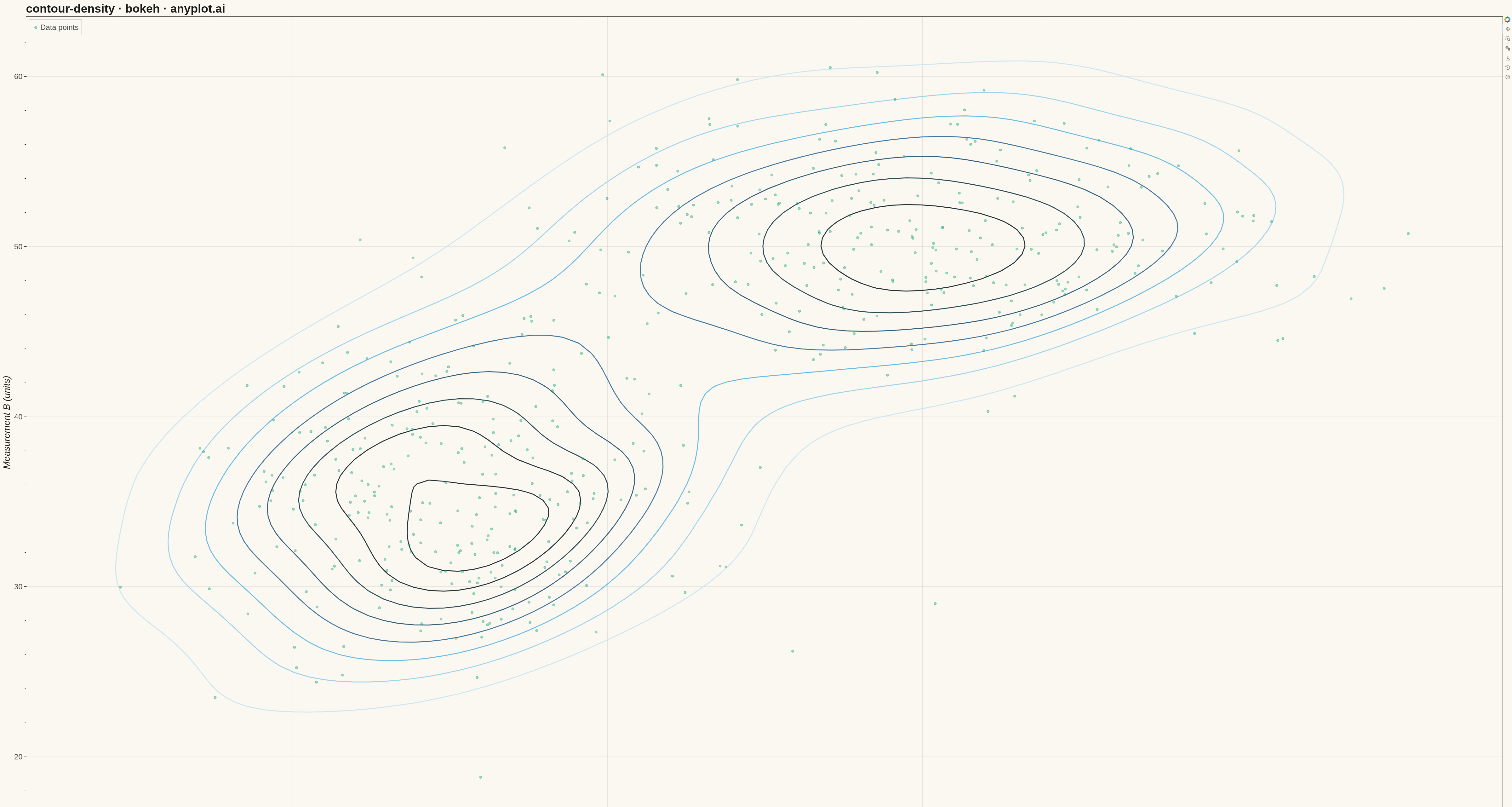
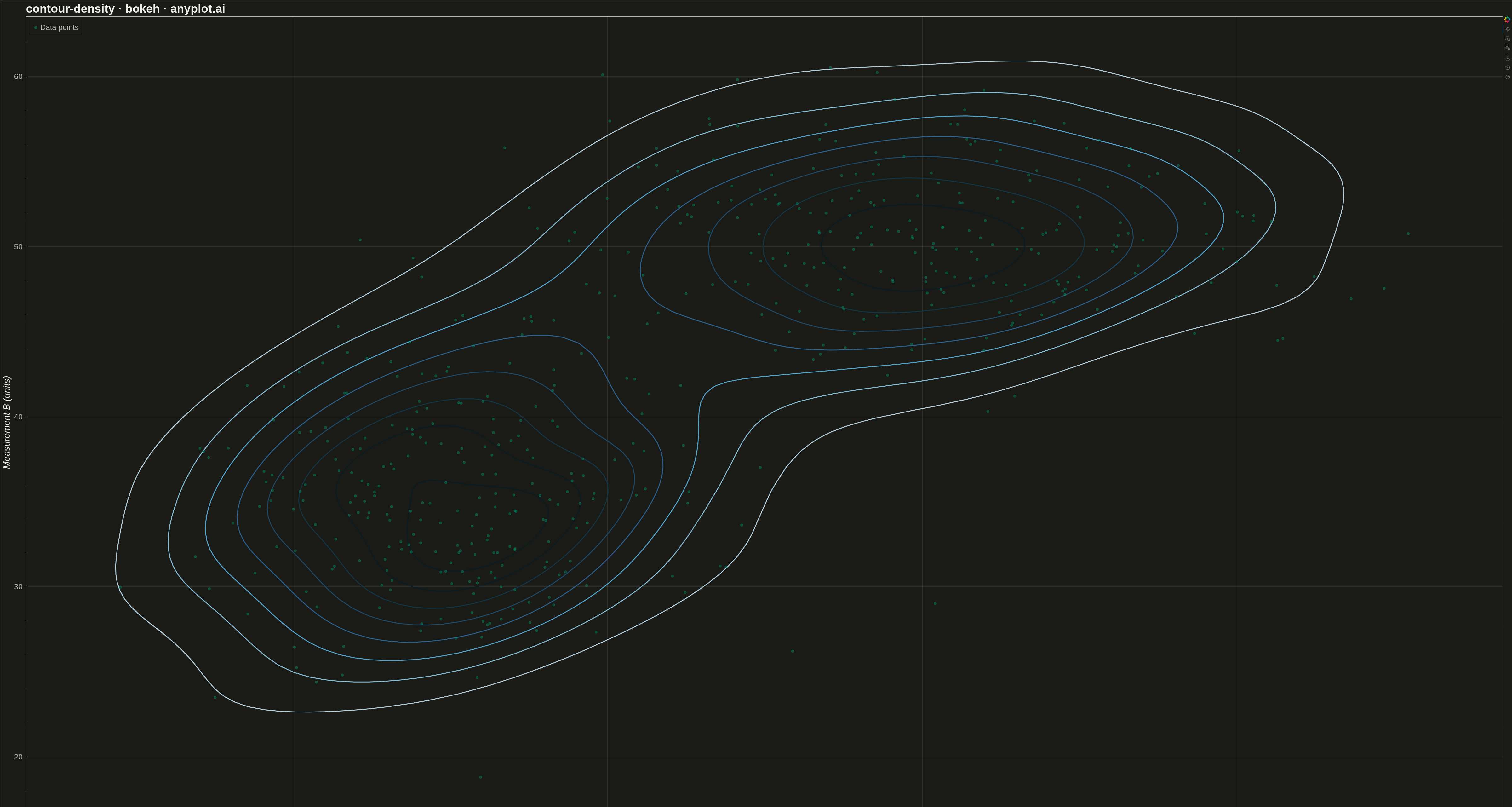
A density contour plot (also known as a 2D KDE contour plot) displays the concentration of points in a 2D scatter plot using contour lines. The contours connect points of equal density, revealing clusters, patterns, and the overall bivariate distribution shape.
""" anyplot.ai
contour-density: Density Contour Plot
Library: bokeh 3.9.0 | Python 3.13.13
Quality: 92/100 | Updated: 2026-05-16
"""

import os
import sys
import time
from pathlib import Path


# Fix import path collision with local library files in same directory
sys.path = [p for p in sys.path if not p.endswith(("bokeh.py", "implementations/python"))]

import numpy as np
from bokeh.io import output_file, save
from bokeh.models import ColumnDataSource
from bokeh.plotting import figure
from scipy import stats
from selenium import webdriver
from selenium.webdriver.chrome.options import Options


mpl_module = __import__("matplotlib")
mpl_module.use("Agg")
plt = __import__("matplotlib.pyplot", fromlist=["pyplot"])

THEME = os.getenv("ANYPLOT_THEME", "light")
PAGE_BG = "#FAF8F1" if THEME == "light" else "#1A1A17"
INK = "#1A1A17" if THEME == "light" else "#F0EFE8"
INK_SOFT = "#4A4A44" if THEME == "light" else "#B8B7B0"
BRAND = "#009E73"

# Data - bivariate distribution with clusters
np.random.seed(42)
n_points = 500

cluster1_x = np.random.normal(25, 4, n_points // 2)
cluster1_y = np.random.normal(35, 5, n_points // 2)
cluster2_x = np.random.normal(40, 6, n_points // 2)
cluster2_y = np.random.normal(50, 4, n_points // 2)

x = np.concatenate([cluster1_x, cluster2_x])
y = np.concatenate([cluster1_y, cluster2_y])

# Compute 2D KDE
kde = stats.gaussian_kde([x, y])

# Create grid for contour evaluation
x_min, x_max = x.min() - 3, x.max() + 3
y_min, y_max = y.min() - 3, y.max() + 3
xx, yy = np.meshgrid(np.linspace(x_min, x_max, 100), np.linspace(y_min, y_max, 100))
positions = np.vstack([xx.ravel(), yy.ravel()])
density = kde(positions).reshape(xx.shape)

# Extract contour lines using matplotlib (for calculation only)
fig_temp, ax_temp = plt.subplots()
contour_set = ax_temp.contour(xx, yy, density, levels=8)
plt.close(fig_temp)

# Create Bokeh figure
p = figure(
    width=4800,
    height=2700,
    title="contour-density · bokeh · anyplot.ai",
    x_axis_label="Measurement A (units)",
    y_axis_label="Measurement B (units)",
    x_range=(x_min, x_max),
    y_range=(y_min, y_max),
)

# Contour colors - blue gradient (low to high density)
colors = ["#e8f4f8", "#c6e4f2", "#94cfea", "#5bb4e0", "#306998", "#1f5070", "#143848", "#0a1c24"]

# Plot contour lines
for i, level_segs in enumerate(contour_set.allsegs):
    color = colors[min(i, len(colors) - 1)]
    for seg in level_segs:
        if len(seg) > 1:
            p.line(x=seg[:, 0], y=seg[:, 1], line_width=3, line_color=color, line_alpha=0.9)

# Overlay scatter points (using Okabe-Ito first series)
source = ColumnDataSource(data={"x": x, "y": y})
p.scatter(x="x", y="y", source=source, size=8, color=BRAND, alpha=0.4, legend_label="Data points")

# Styling
p.title.text_font_size = "28pt"
p.title.text_color = INK
p.xaxis.axis_label_text_font_size = "22pt"
p.yaxis.axis_label_text_font_size = "22pt"
p.xaxis.axis_label_text_color = INK
p.yaxis.axis_label_text_color = INK
p.xaxis.major_label_text_font_size = "18pt"
p.yaxis.major_label_text_font_size = "18pt"
p.xaxis.major_label_text_color = INK_SOFT
p.yaxis.major_label_text_color = INK_SOFT

p.background_fill_color = PAGE_BG
p.border_fill_color = PAGE_BG
p.outline_line_color = INK_SOFT
p.xaxis.axis_line_color = INK_SOFT
p.yaxis.axis_line_color = INK_SOFT

p.xgrid.grid_line_color = INK
p.ygrid.grid_line_color = INK
p.xgrid.grid_line_alpha = 0.10
p.ygrid.grid_line_alpha = 0.10

p.legend.label_text_font_size = "18pt"
p.legend.location = "top_left"
p.legend.label_text_color = INK_SOFT
p.legend.background_fill_color = PAGE_BG
p.legend.border_line_color = INK_SOFT

# Save HTML
output_file(f"plot-{THEME}.html")
save(p)

# Screenshot with Selenium
W, H = 4800, 2700
opts = Options()
for arg in (
    "--headless=new",
    "--no-sandbox",
    "--disable-dev-shm-usage",
    "--disable-gpu",
    f"--window-size={W},{H}",
    "--hide-scrollbars",
):
    opts.add_argument(arg)
driver = webdriver.Chrome(options=opts)
driver.set_window_size(W, H)
driver.get(f"file://{Path(f'plot-{THEME}.html').resolve()}")
time.sleep(3)
driver.save_screenshot(f"plot-{THEME}.png")
driver.quit()
Runnable source as JSON, for any HTTP client: https://api.anyplot.ai/specs/contour-density/bokeh/code. Any spec id and library id listed in llms-full.txt fit the same URL shape; every URL below is complete and callable.
{
  "spec_id": "contour-density",
  "language": "python",
  "library": "bokeh",
  "page": "https://anyplot.ai/contour-density/python/bokeh",
  "hub": "https://anyplot.ai/contour-density",
  "code_json": "https://api.anyplot.ai/specs/contour-density/bokeh/code",
  "spec_json": "https://api.anyplot.ai/specs/contour-density",
  "render_light_png": "https://storage.googleapis.com/anyplot-images/plots/contour-density/python/bokeh/plot-light.png",
  "render_dark_png": "https://storage.googleapis.com/anyplot-images/plots/contour-density/python/bokeh/plot-dark.png",
  "interactive_light_html": "https://storage.googleapis.com/anyplot-images/plots/contour-density/python/bokeh/plot-light.html",
  "interactive_dark_html": "https://storage.googleapis.com/anyplot-images/plots/contour-density/python/bokeh/plot-dark.html",
  "quality_score": 92.0,
  "license": "MIT",
  "guide": "https://anyplot.ai/llms.txt"
}
Part of Density Contour Plot on anyplot.ai.