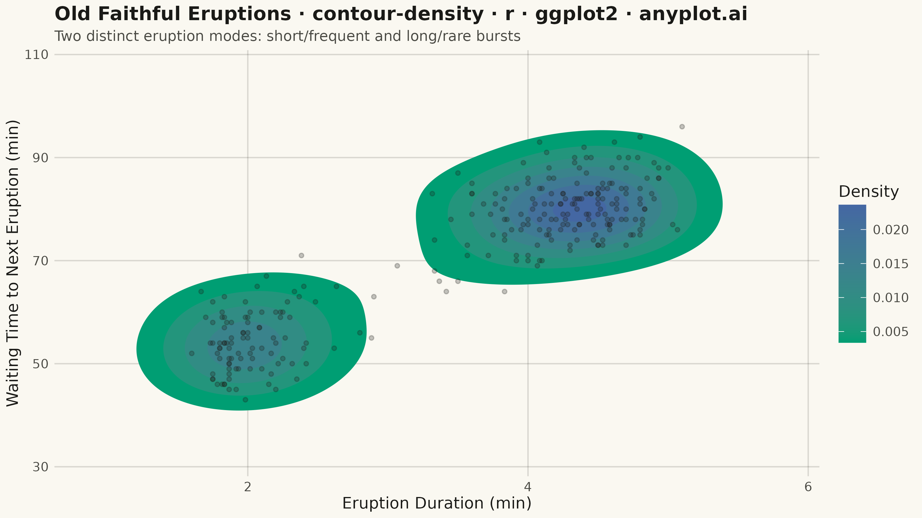
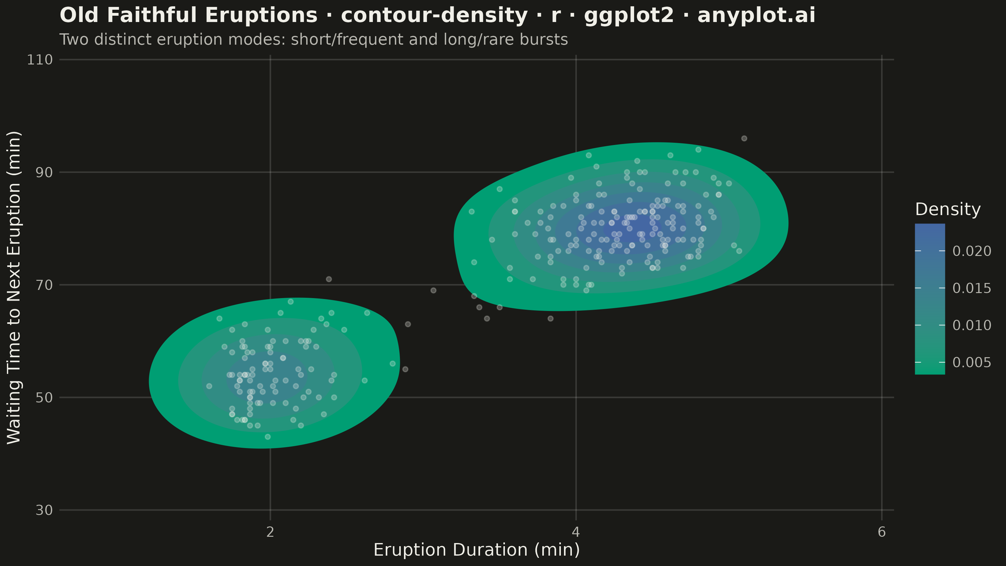
The same plot in 14 other libraries — Python: Altair, Bokeh, lets-plot, Matplotlib, Plotly, plotnine, Pygal, Seaborn; Julia: Makie.jl; JavaScript: Chart.js, D3.js, Apache ECharts, Highcharts, MUI X Charts. Compare all 15 side by side: Density Contour Plot in Python, R, Julia and JavaScript.
A density contour plot (also known as a 2D KDE contour plot) displays the concentration of points in a 2D scatter plot using contour lines. The contours connect points of equal density, revealing clusters, patterns, and the overall bivariate distribution shape.
#' anyplot.ai
#' contour-density: Density Contour Plot
#' Library: ggplot2 3.5.1 | R 4.4.1
#' Quality: 89/100 | Created: 2026-09-04

library(ggplot2)
library(ragg)
library(scales)

set.seed(42)

# --- Theme tokens -------------------------------------------------------
THEME    <- Sys.getenv("ANYPLOT_THEME", "light")
PAGE_BG  <- if (THEME == "light") "#FAF8F1" else "#1A1A17"
INK      <- if (THEME == "light") "#1A1A17" else "#F0EFE8"
INK_SOFT <- if (THEME == "light") "#4A4A44" else "#B8B7B0"

# --- Data -----------------------------------------------------------------
# Old Faithful geyser: eruption duration vs. waiting time until the next
# eruption. The bivariate distribution is famously bimodal, which makes it a
# clean showcase for density contours (short/frequent vs. long/rare bursts).
df <- data.frame(
  eruption_duration = faithful$eruptions,
  waiting_time      = faithful$waiting
)

# stat_density_2d evaluates its KDE grid exactly over the trained scale
# range (ggplot2 passes `scales$x$dimension()` straight to MASS::kde2d's
# `lims`), so a data point sitting right at the min/max of that range
# leaves no room for its contour to close and the outermost isoband gets
# cut into a jagged notch. The smaller cluster is tighter than the overall
# spread that the shared bandwidth is fit to, so 8% slack was not enough
# room for its isoband to taper to zero before hitting the grid edge;
# 25% is enough for both clusters to close cleanly.
x_rng  <- range(df$eruption_duration)
y_rng  <- range(df$waiting_time)
x_pad  <- diff(x_rng) * 0.25
y_pad  <- diff(y_rng) * 0.25

# --- Plot -------------------------------------------------------------------
p <- ggplot(df, aes(x = eruption_duration, y = waiting_time)) +
  stat_density_2d(
    aes(fill = after_stat(level)),
    geom        = "polygon",
    color       = NA,
    contour_var = "density",
    n           = 300,
    bins        = 8
  ) +
  geom_point(color = INK, size = 1.0, alpha = 0.25) +
  scale_fill_gradient(low = "#009E73", high = "#4467A3", name = "Density") +
  scale_x_continuous(limits = c(x_rng[1] - x_pad, x_rng[2] + x_pad), expand = expansion(mult = 0.02)) +
  scale_y_continuous(limits = c(y_rng[1] - y_pad, y_rng[2] + y_pad), expand = expansion(mult = 0.02)) +
  labs(
    title    = "Old Faithful Eruptions · contour-density · r · ggplot2 · anyplot.ai",
    subtitle = "Two distinct eruption modes: short/frequent and long/rare bursts",
    x        = "Eruption Duration (min)",
    y        = "Waiting Time to Next Eruption (min)"
  ) +
  theme_minimal(base_size = 8) +
  theme(
    plot.background   = element_rect(fill = PAGE_BG, color = PAGE_BG),
    panel.background  = element_rect(fill = PAGE_BG, color = NA),
    panel.grid.major  = element_line(color = scales::alpha(INK, 0.15), linewidth = 0.4),
    panel.grid.minor  = element_blank(),
    axis.title        = element_text(color = INK, size = 10),
    axis.text         = element_text(color = INK_SOFT, size = 8),
    axis.ticks        = element_blank(),
    plot.title        = element_text(color = INK, size = 12, face = "bold"),
    plot.subtitle     = element_text(color = INK_SOFT, size = 9),
    legend.title      = element_text(color = INK, size = 10),
    legend.text       = element_text(color = INK_SOFT, size = 8),
    legend.background = element_blank(),
    legend.key        = element_blank()
  )

# --- Save -------------------------------------------------------------------
ggsave(
  filename = sprintf("plot-%s.png", THEME),
  plot     = p,
  device   = ragg::agg_png,
  width    = 8,
  height   = 4.5,
  units    = "in",
  dpi      = 400
)
Runnable source as JSON, for any HTTP client: https://api.anyplot.ai/specs/contour-density/ggplot2/code. Any spec id and library id listed in llms-full.txt fit the same URL shape; every URL below is complete and callable.
{
  "spec_id": "contour-density",
  "language": "r",
  "library": "ggplot2",
  "page": "https://anyplot.ai/contour-density/r/ggplot2",
  "hub": "https://anyplot.ai/contour-density",
  "code_json": "https://api.anyplot.ai/specs/contour-density/ggplot2/code",
  "spec_json": "https://api.anyplot.ai/specs/contour-density",
  "render_light_png": "https://storage.googleapis.com/anyplot-images/plots/contour-density/r/ggplot2/plot-light.png",
  "render_dark_png": "https://storage.googleapis.com/anyplot-images/plots/contour-density/r/ggplot2/plot-dark.png",
  "quality_score": 89.0,
  "license": "MIT",
  "guide": "https://anyplot.ai/llms.txt"
}
Part of Density Contour Plot on anyplot.ai.