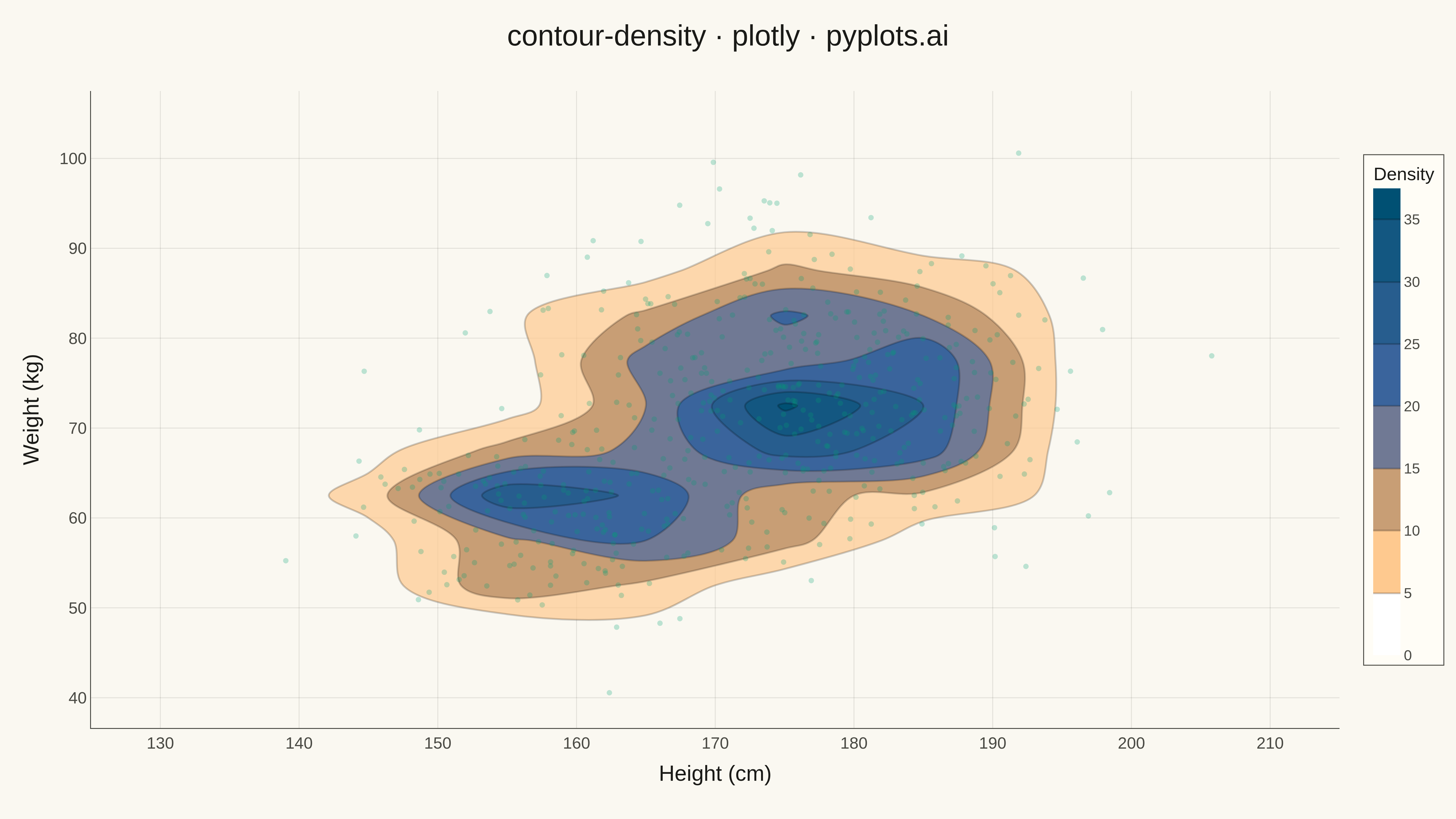
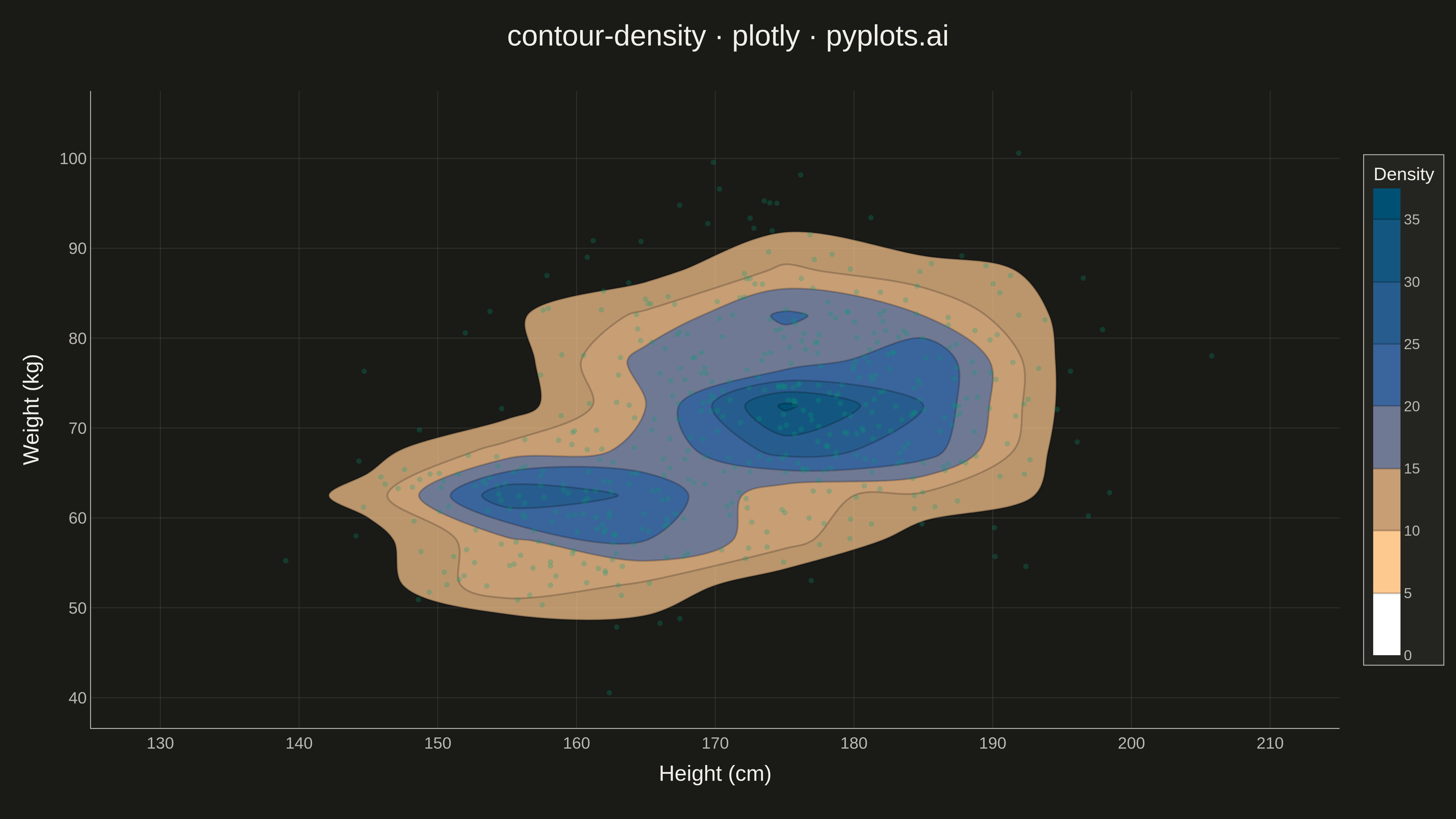
A density contour plot (also known as a 2D KDE contour plot) displays the concentration of points in a 2D scatter plot using contour lines. The contours connect points of equal density, revealing clusters, patterns, and the overall bivariate distribution shape.
""" anyplot.ai
contour-density: Density Contour Plot
Library: plotly 6.7.0 | Python 3.13.13
Quality: 95/100 | Updated: 2026-05-16
"""

import os

import numpy as np
import plotly.graph_objects as go


# Theme tokens (see prompts/default-style-guide.md)
THEME = os.getenv("ANYPLOT_THEME", "light")
PAGE_BG = "#FAF8F1" if THEME == "light" else "#1A1A17"
ELEVATED_BG = "#FFFDF6" if THEME == "light" else "#242420"
INK = "#1A1A17" if THEME == "light" else "#F0EFE8"
INK_SOFT = "#4A4A44" if THEME == "light" else "#B8B7B0"
GRID = "rgba(26,26,23,0.10)" if THEME == "light" else "rgba(240,239,232,0.10)"

# Data - bivariate distribution with three clusters
np.random.seed(42)

# Create three clusters with realistic domain context (height vs weight measurements)
n_points = 500

# Cluster 1: Lighter individuals
cluster1_x = np.random.normal(160, 8, n_points // 3)  # Height in cm
cluster1_y = np.random.normal(60, 6, n_points // 3)  # Weight in kg

# Cluster 2: Heavier individuals
cluster2_x = np.random.normal(175, 10, n_points // 3)
cluster2_y = np.random.normal(80, 8, n_points // 3)

# Cluster 3: Tall but lighter individuals
cluster3_x = np.random.normal(180, 7, n_points // 3)
cluster3_y = np.random.normal(70, 7, n_points // 3)

x = np.concatenate([cluster1_x, cluster2_x, cluster3_x])
y = np.concatenate([cluster1_y, cluster2_y, cluster3_y])

# Define theme-aware colorscale for density (continuous data)
# Use viridis-like progression that works on both light and dark backgrounds
colorscale = [
    [0, "rgba(255,255,255,0)"],  # Transparent at low density
    [0.2, "#FDB462"],  # Light orange (visible on both themes)
    [0.5, "#4467A3"],  # Blue (Okabe-Ito position 3)
    [1, "#005073"],  # Dark blue (increased contrast)
]

# Create figure with density contour
fig = go.Figure()

# Add density contour plot with interactive hover
fig.add_trace(
    go.Histogram2dContour(
        x=x,
        y=y,
        colorscale=colorscale,
        contours=dict(showlabels=False, coloring="fill"),
        ncontours=14,
        showscale=True,
        colorbar=dict(
            title=dict(text="Density", font=dict(size=20, color=INK)),
            tickfont=dict(size=16, color=INK_SOFT),
            len=0.8,
            bgcolor=ELEVATED_BG,
            bordercolor=INK_SOFT,
            borderwidth=1,
        ),
        line=dict(width=2, color="rgba(0,0,0,0.2)"),
        hovertemplate="<b>Density Region</b><br>Height: %{x:.1f} cm<br>Weight: %{y:.1f} kg<extra></extra>",
    )
)

# Add scatter points for context (semi-transparent, interactive)
fig.add_trace(
    go.Scatter(
        x=x,
        y=y,
        mode="markers",
        marker=dict(
            size=6,
            color="#009E73",  # Okabe-Ito position 1 (brand color, theme-independent)
            opacity=0.25,
            line=dict(width=0),
        ),
        showlegend=False,
        name="Individual measurements",
        hovertemplate="<b>Measurement</b><br>Height: %{x:.1f} cm<br>Weight: %{y:.1f} kg<extra></extra>",
    )
)

# Update layout with theme-adaptive styling
fig.update_layout(
    title=dict(text="contour-density · plotly · pyplots.ai", font=dict(size=32, color=INK), x=0.5, xanchor="center"),
    xaxis=dict(
        title=dict(text="Height (cm)", font=dict(size=24, color=INK)),
        tickfont=dict(size=18, color=INK_SOFT),
        showgrid=True,
        gridcolor=GRID,
        gridwidth=1,
        linecolor=INK_SOFT,
        zerolinecolor=INK_SOFT,
    ),
    yaxis=dict(
        title=dict(text="Weight (kg)", font=dict(size=24, color=INK)),
        tickfont=dict(size=18, color=INK_SOFT),
        showgrid=True,
        gridcolor=GRID,
        gridwidth=1,
        linecolor=INK_SOFT,
        zerolinecolor=INK_SOFT,
    ),
    paper_bgcolor=PAGE_BG,
    plot_bgcolor=PAGE_BG,
    font=dict(color=INK),
    width=1600,
    height=900,
    margin=dict(l=100, r=120, t=100, b=100),
    hovermode="closest",
)

# Save as PNG and HTML with theme-suffixed filenames
fig.write_image(f"plot-{THEME}.png", width=1600, height=900, scale=3)
fig.write_html(f"plot-{THEME}.html", include_plotlyjs="cdn")
Runnable source as JSON, for any HTTP client: https://api.anyplot.ai/specs/contour-density/plotly/code. Any spec id and library id listed in llms-full.txt fit the same URL shape; every URL below is complete and callable.
{
  "spec_id": "contour-density",
  "language": "python",
  "library": "plotly",
  "page": "https://anyplot.ai/contour-density/python/plotly",
  "hub": "https://anyplot.ai/contour-density",
  "code_json": "https://api.anyplot.ai/specs/contour-density/plotly/code",
  "spec_json": "https://api.anyplot.ai/specs/contour-density",
  "render_light_png": "https://storage.googleapis.com/anyplot-images/plots/contour-density/python/plotly/plot-light.png",
  "render_dark_png": "https://storage.googleapis.com/anyplot-images/plots/contour-density/python/plotly/plot-dark.png",
  "interactive_light_html": "https://storage.googleapis.com/anyplot-images/plots/contour-density/python/plotly/plot-light.html",
  "interactive_dark_html": "https://storage.googleapis.com/anyplot-images/plots/contour-density/python/plotly/plot-dark.html",
  "quality_score": 95.0,
  "license": "MIT",
  "guide": "https://anyplot.ai/llms.txt"
}
Part of Density Contour Plot on anyplot.ai.