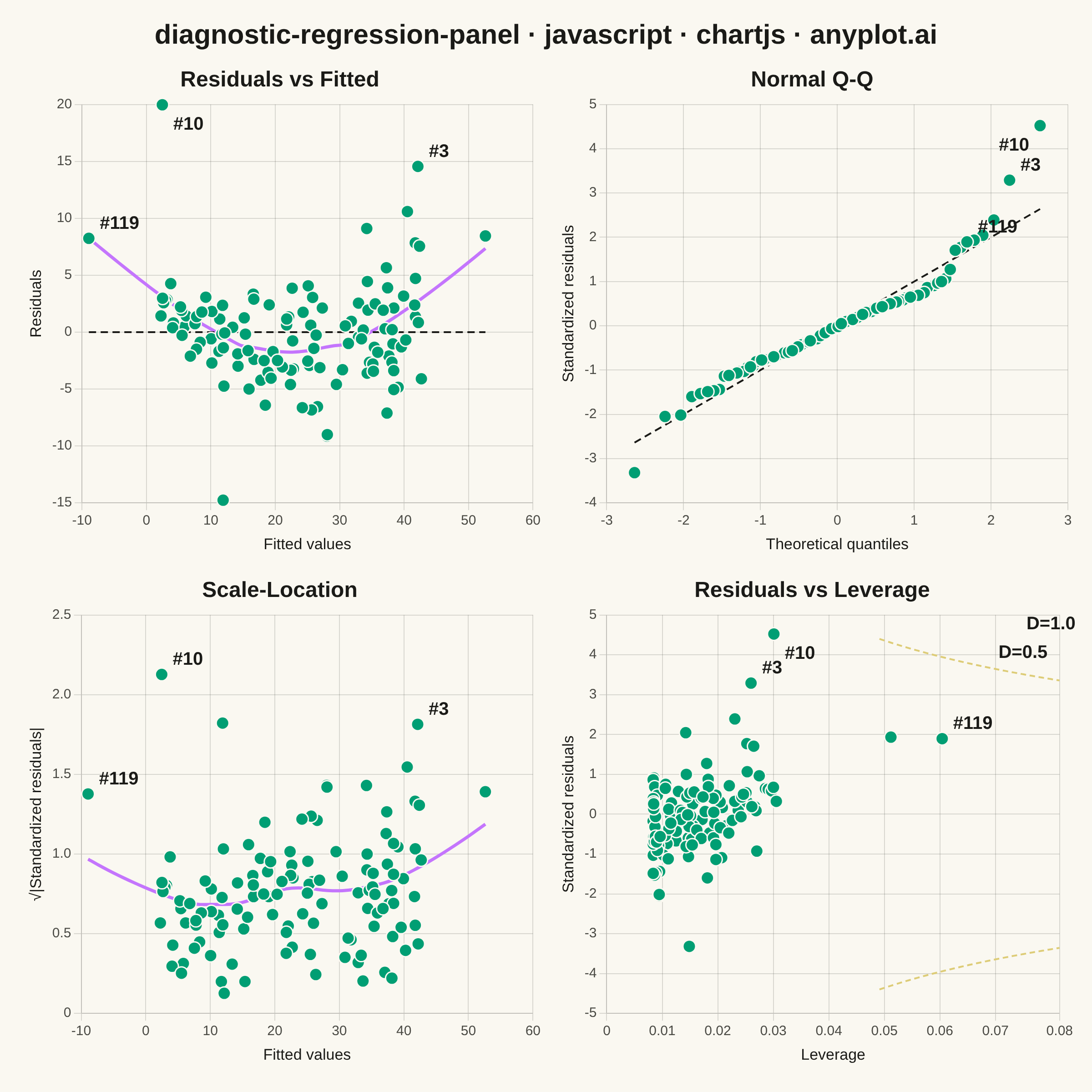
The same plot in 14 other libraries — JavaScript: D3.js, Apache ECharts, Highcharts, MUI X Charts; Python: Altair, Bokeh, lets-plot, Matplotlib, Plotly, plotnine, Pygal, Seaborn; R: ggplot2; Julia: Makie.jl. Compare all 15 side by side: Regression Diagnostic Panel (Four-Plot Display) in Python, R, Julia and JavaScript.
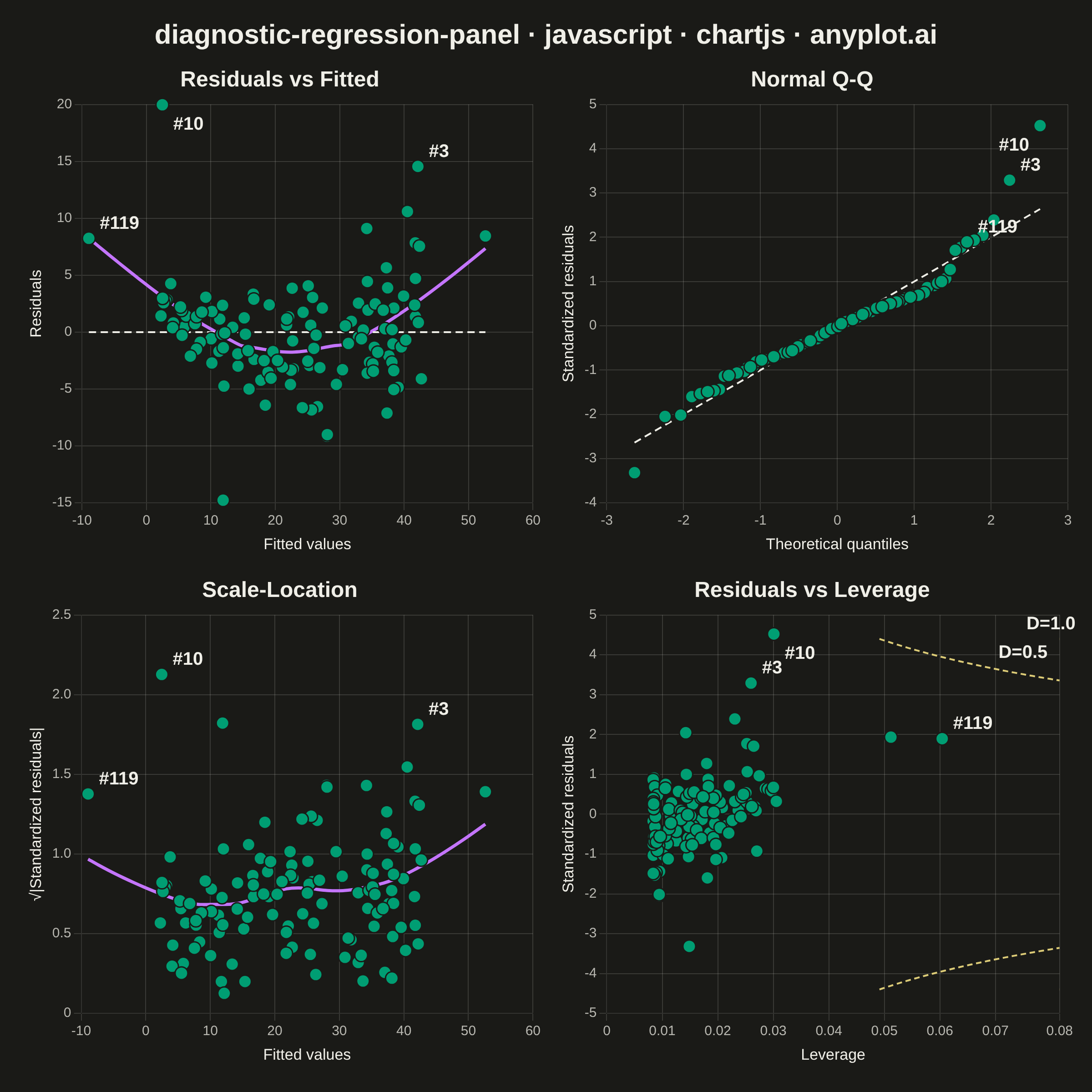
A 2x2 panel of diagnostic plots for evaluating linear regression model assumptions, replicating the classic output of R's `plot(lm)`. The four subplots are: (1) Residuals vs Fitted values to detect non-linearity and heteroscedasticity, (2) Normal Q-Q plot of standardized residuals to assess normality, (3) Scale-Location plot (square root of standardized residuals vs fitted values) to check homoscedasticity, and (4) Residuals vs Leverage with Cook's distance contours to identify influential observations. This composite display is the standard first step in regression model validation across statistics, academia, and regulated industries.
// anyplot.ai
// diagnostic-regression-panel: Regression Diagnostic Panel (Four-Plot Display)
// Library: chartjs 4.4.7 | JavaScript 22.23.2
// Quality: 90/100 | Updated: 2026-09-05

//# anyplot-orientation: square

const t = window.ANYPLOT_TOKENS;
const FONT = "-apple-system, BlinkMacSystemFont, 'Segoe UI', Roboto, Helvetica, Arial, sans-serif";

// --- Deterministic PRNG (LCG) + Box-Muller normal draws ---------------------
function makeLcg(seed) {
  let state = seed >>> 0;
  return function lcg() {
    state = (1103515245 * state + 12345) >>> 0;
    return state / 4294967296;
  };
}
const rand = makeLcg(42);
function randNormal() {
  const u1 = Math.max(rand(), 1e-12);
  const u2 = rand();
  return Math.sqrt(-2 * Math.log(u1)) * Math.cos(2 * Math.PI * u2);
}

// --- Inverse standard-normal CDF (Acklam's rational approximation) ---------
function probit(p) {
  const a = [-3.969683028665376e1, 2.209460984245205e2, -2.759285104469687e2, 1.38357751867269e2, -3.066479806614716e1, 2.506628277459239];
  const b = [-5.447609879822406e1, 1.615858368580409e2, -1.556989798598866e2, 6.680131188771972e1, -1.328068155288572e1];
  const c = [-7.784894002430293e-3, -3.223964580411365e-1, -2.400758277161838, -2.549732539343734, 4.374664141464968, 2.938163982698783];
  const d = [7.784695709041462e-3, 3.224671290700398e-1, 2.445134137142996, 3.754408661907416];
  const plow = 0.02425;
  const phigh = 1 - plow;
  if (p < plow) {
    const q = Math.sqrt(-2 * Math.log(p));
    return (((((c[0] * q + c[1]) * q + c[2]) * q + c[3]) * q + c[4]) * q + c[5]) / ((((d[0] * q + d[1]) * q + d[2]) * q + d[3]) * q + 1);
  }
  if (p <= phigh) {
    const q = p - 0.5;
    const r = q * q;
    return ((((((a[0] * r + a[1]) * r + a[2]) * r + a[3]) * r + a[4]) * r + a[5]) * q) / (((((b[0] * r + b[1]) * r + b[2]) * r + b[3]) * r + b[4]) * r + 1);
  }
  const q = Math.sqrt(-2 * Math.log(1 - p));
  return -(((((c[0] * q + c[1]) * q + c[2]) * q + c[3]) * q + c[4]) * q + c[5]) / ((((d[0] * q + d[1]) * q + d[2]) * q + d[3]) * q + 1);
}

// --- LOWESS smoother: tricube-weighted local linear regression -------------
function lowess(xs, ys, fracSpan, gridSize) {
  const n = xs.length;
  const order = xs.map((_, i) => i).sort((i, j) => xs[i] - xs[j]);
  const sx = order.map((i) => xs[i]);
  const sy = order.map((i) => ys[i]);
  const bandwidth = Math.max(2, Math.round(fracSpan * n));
  const xmin = sx[0];
  const xmax = sx[n - 1];
  const grid = [];
  for (let g = 0; g < gridSize; g++) grid.push(xmin + ((xmax - xmin) * g) / (gridSize - 1));
  return grid.map((x0) => {
    const dists = sx.map((xi) => Math.abs(xi - x0));
    const h = [...dists].sort((p, q) => p - q)[Math.min(bandwidth, n - 1)] || 1e-6;
    let sw = 0;
    let swx = 0;
    let swy = 0;
    let swxx = 0;
    let swxy = 0;
    for (let i = 0; i < n; i++) {
      const u = dists[i] / h;
      if (u >= 1) continue;
      const w = (1 - u * u * u) ** 3;
      sw += w;
      swx += w * sx[i];
      swy += w * sy[i];
      swxx += w * sx[i] * sx[i];
      swxy += w * sx[i] * sy[i];
    }
    const denom = sw * swxx - swx * swx;
    let slope = 0;
    let intercept = swy / sw;
    if (Math.abs(denom) > 1e-9) {
      slope = (sw * swxy - swx * swy) / denom;
      intercept = (swy - slope * swx) / sw;
    }
    return { x: x0, y: intercept + slope * x0 };
  });
}

// --- Data: simulate a fitted regression with mild non-linearity, -----------
// heteroscedastic noise, and a few high-leverage / high-influence points ----
const n = 120;
const x = [];
for (let i = 0; i < n; i++) x.push(rand() * 10);
x[n - 2] = 12.4; // high-leverage points (sparse, far from the predictor mean)
x[n - 1] = -2.6;

const y = x.map((xi) => {
  const trueSignal = 5 + 2.2 * xi + 0.18 * xi * xi; // mild curvature the linear fit misses
  const noiseScale = 1 + 0.35 * Math.abs(xi); // heteroscedastic spread
  return trueSignal + randNormal() * noiseScale;
});
y[10] += 19; // outliers that become influential once combined with leverage
y[45] -= 16;

// --- Simple OLS fit: y = b0 + b1 * x ----------------------------------------
const xbar = x.reduce((s, v) => s + v, 0) / n;
const ybar = y.reduce((s, v) => s + v, 0) / n;
const sxx = x.reduce((s, xi) => s + (xi - xbar) ** 2, 0);
const sxy = x.reduce((s, xi, i) => s + (xi - xbar) * (y[i] - ybar), 0);
const b1 = sxy / sxx;
const b0 = ybar - b1 * xbar;

const fitted = x.map((xi) => b0 + b1 * xi);
const residuals = y.map((yi, i) => yi - fitted[i]);
const p = 2; // estimated parameters (intercept + slope)
const rss = residuals.reduce((s, r) => s + r * r, 0);
const sigma = Math.sqrt(rss / (n - p));

const leverage = x.map((xi) => 1 / n + (xi - xbar) ** 2 / sxx);
const stdResiduals = residuals.map((r, i) => r / (sigma * Math.sqrt(1 - leverage[i])));
const sqrtAbsStd = stdResiduals.map((r) => Math.sqrt(Math.abs(r)));
const cooksD = stdResiduals.map((sr, i) => (sr * sr * leverage[i]) / ((1 - leverage[i]) * p));

// The 3 most influential observations (highest Cook's distance) — labeled in every panel
const topInfluential = cooksD
  .map((d, i) => [d, i])
  .sort((a, b) => b[0] - a[0])
  .slice(0, 3)
  .map(([, i]) => i);

// Q-Q coordinates: sort standardized residuals, pair with theoretical normal quantiles
const qqOrder = stdResiduals.map((_, i) => i).sort((i, j) => stdResiduals[i] - stdResiduals[j]);
const qqByIndex = new Array(n);
qqOrder.forEach((origIdx, rank) => {
  const pval = (rank + 0.5) / n;
  qqByIndex[origIdx] = { x: probit(pval), y: stdResiduals[origIdx] };
});
const qqTheoretical = qqByIndex.map((pt) => pt.x);
const qqMin = Math.min(...qqTheoretical);
const qqMax = Math.max(...qqTheoretical);

// Cook's distance contours for the Residuals-vs-Leverage panel
const axisYMax = 5; // a little headroom above the data so markers never clip the frame
const contourClip = 4.4;
const maxLeverage = Math.max(...leverage);
const leverageAxisMax = maxLeverage * 1.35;
function cookContour(D) {
  const hMin = (D * p) / (D * p + contourClip * contourClip);
  const steps = 40;
  const pos = [];
  for (let i = 0; i <= steps; i++) {
    const h = hMin + ((leverageAxisMax - hMin) * i) / steps;
    if (h <= 0 || h >= 1) continue;
    pos.push({ x: h, y: Math.min(Math.sqrt((D * p * (1 - h)) / h), contourClip) });
  }
  return { pos, neg: pos.map((pt) => ({ x: pt.x, y: -pt.y })) };
}
const cook05 = cookContour(0.5);
const cook10 = cookContour(1.0);

// --- Consistent scatter marker styling across all four subplots ------------
const POINT_STYLE = {
  backgroundColor: t.palette[0],
  borderColor: t.pageBg,
  borderWidth: 1.5,
  radius: 7,
  hoverRadius: 7,
};
const SMOOTH_COLOR = t.palette[1];
const REFERENCE_COLOR = t.ink;
const CONTOUR_COLOR = t.amber;

// --- Point-label plugin: draws "#idx" next to the top-influence points -----
// Flips the label to the opposite side of the point whenever the default
// placement (upper-right) would run past the chart area — into the panel
// title above, or off the right/left edge of the canvas.
function labelPlugin(getPoints) {
  return {
    id: "anyplotPointLabels",
    afterDatasetsDraw(chart) {
      const { ctx, scales, chartArea } = chart;
      ctx.save();
      ctx.font = "600 20px " + FONT;
      ctx.fillStyle = t.ink;
      ctx.textAlign = "left";
      ctx.textBaseline = "middle";
      getPoints().forEach(({ x, y, label }) => {
        const px = scales.x.getPixelForValue(x);
        const py = scales.y.getPixelForValue(y);
        const w = ctx.measureText(label).width;
        const nearTop = py - 26 < chartArea.top;
        const nearRight = px + 12 + w > chartArea.right;
        const lx = nearRight ? px - 12 - w : px + 12;
        const ly = nearTop ? py + 22 : py - 16;
        ctx.fillText(label, lx, ly);
      });
      ctx.restore();
    },
  };
}

// --- Shared chrome for every subplot ----------------------------------------
function baseOptions(panelTitle, xLabel, yLabel, extraScales) {
  return {
    responsive: true,
    maintainAspectRatio: false,
    animation: false,
    layout: { padding: 8 },
    plugins: {
      legend: { display: false },
      title: { display: true, text: panelTitle, color: t.ink, font: { size: 24, weight: "600", family: FONT }, padding: { bottom: 12 } },
    },
    scales: {
      x: {
        ticks: { color: t.inkSoft, font: { size: 15, family: FONT } },
        grid: { color: t.grid },
        title: { display: true, text: xLabel, color: t.ink, font: { size: 17, family: FONT } },
        ...(extraScales?.x || {}),
      },
      y: {
        ticks: { color: t.inkSoft, font: { size: 15, family: FONT } },
        grid: { color: t.grid },
        title: { display: true, text: yLabel, color: t.ink, font: { size: 17, family: FONT } },
        ...(extraScales?.y || {}),
      },
    },
  };
}

// --- Mount: shared title above a 2x2 grid of independent Chart.js charts ---
const root = document.createElement("div");
document.getElementById("container").appendChild(root);
root.style.display = "flex";
root.style.flexDirection = "column";
root.style.width = "100%";
root.style.height = "100%";
root.style.backgroundColor = t.pageBg;

const titleEl = document.createElement("div");
titleEl.textContent = "diagnostic-regression-panel · javascript · chartjs · anyplot.ai";
titleEl.style.textAlign = "center";
titleEl.style.color = t.ink;
titleEl.style.fontFamily = FONT;
titleEl.style.fontWeight = "700";
titleEl.style.fontSize = "30px";
titleEl.style.padding = "22px 0 10px 0";
root.appendChild(titleEl);

const grid = document.createElement("div");
grid.style.flex = "1 1 auto";
grid.style.display = "grid";
grid.style.gridTemplateColumns = "1fr 1fr";
grid.style.gridTemplateRows = "1fr 1fr";
grid.style.columnGap = "6px";
grid.style.rowGap = "6px";
grid.style.minHeight = "0";
grid.style.padding = "0 18px 18px 18px";
root.appendChild(grid);

function addCanvas() {
  const cell = document.createElement("div");
  cell.style.position = "relative";
  cell.style.minWidth = "0";
  cell.style.minHeight = "0";
  grid.appendChild(cell);
  const canvas = document.createElement("canvas");
  cell.appendChild(canvas);
  return canvas;
}

// --- Panel 1: Residuals vs Fitted -------------------------------------------
const fittedMin = Math.min(...fitted);
const fittedMax = Math.max(...fitted);
const lowess1 = lowess(fitted, residuals, 0.6, 40);
new Chart(addCanvas(), {
  type: "scatter",
  data: {
    datasets: [
      { data: fitted.map((f, i) => ({ x: f, y: residuals[i] })), ...POINT_STYLE, showLine: false },
      { data: [{ x: fittedMin, y: 0 }, { x: fittedMax, y: 0 }], showLine: true, borderColor: REFERENCE_COLOR, borderWidth: 2, borderDash: [8, 5], pointRadius: 0 },
      { data: lowess1, showLine: true, borderColor: SMOOTH_COLOR, borderWidth: 3.5, pointRadius: 0, tension: 0.25 },
    ],
  },
  options: baseOptions("Residuals vs Fitted", "Fitted values", "Residuals"),
  plugins: [labelPlugin(() => topInfluential.map((i) => ({ x: fitted[i], y: residuals[i], label: `#${i}` })))],
});

// --- Panel 2: Normal Q-Q -----------------------------------------------------
new Chart(addCanvas(), {
  type: "scatter",
  data: {
    datasets: [
      { data: qqByIndex.map((pt) => ({ x: pt.x, y: pt.y })), ...POINT_STYLE, showLine: false },
      { data: [{ x: qqMin, y: qqMin }, { x: qqMax, y: qqMax }], showLine: true, borderColor: REFERENCE_COLOR, borderWidth: 2, borderDash: [8, 5], pointRadius: 0 },
    ],
  },
  options: baseOptions("Normal Q-Q", "Theoretical quantiles", "Standardized residuals"),
  plugins: [labelPlugin(() => topInfluential.map((i) => ({ x: qqByIndex[i].x, y: qqByIndex[i].y, label: `#${i}` })))],
});

// --- Panel 3: Scale-Location --------------------------------------------------
const lowess3 = lowess(fitted, sqrtAbsStd, 0.6, 40);
new Chart(addCanvas(), {
  type: "scatter",
  data: {
    datasets: [
      { data: fitted.map((f, i) => ({ x: f, y: sqrtAbsStd[i] })), ...POINT_STYLE, showLine: false },
      { data: lowess3, showLine: true, borderColor: SMOOTH_COLOR, borderWidth: 3.5, pointRadius: 0, tension: 0.25 },
    ],
  },
  options: baseOptions("Scale-Location", "Fitted values", "√|Standardized residuals|", { y: { min: 0 } }),
  plugins: [labelPlugin(() => topInfluential.map((i) => ({ x: fitted[i], y: sqrtAbsStd[i], label: `#${i}` })))],
});

// --- Panel 4: Residuals vs Leverage (with Cook's distance contours) --------
new Chart(addCanvas(), {
  type: "scatter",
  data: {
    datasets: [
      { data: leverage.map((h, i) => ({ x: h, y: stdResiduals[i] })), ...POINT_STYLE, showLine: false },
      { data: cook05.pos, showLine: true, borderColor: CONTOUR_COLOR, borderWidth: 2, borderDash: [6, 4], pointRadius: 0, tension: 0.15 },
      { data: cook05.neg, showLine: true, borderColor: CONTOUR_COLOR, borderWidth: 2, borderDash: [6, 4], pointRadius: 0, tension: 0.15 },
      { data: cook10.pos, showLine: true, borderColor: CONTOUR_COLOR, borderWidth: 2.5, pointRadius: 0, tension: 0.15 },
      { data: cook10.neg, showLine: true, borderColor: CONTOUR_COLOR, borderWidth: 2.5, pointRadius: 0, tension: 0.15 },
    ],
  },
  options: baseOptions("Residuals vs Leverage", "Leverage", "Standardized residuals", {
    x: { min: 0, max: leverageAxisMax },
    y: { min: -axisYMax, max: axisYMax },
  }),
  plugins: [
    labelPlugin(() => {
      const mid05 = cook05.pos[Math.floor(cook05.pos.length * 0.6)];
      const mid10 = cook10.pos[Math.floor(cook10.pos.length * 0.6)];
      return [
        ...topInfluential.map((i) => ({ x: leverage[i], y: stdResiduals[i], label: `#${i}` })),
        { x: mid05.x, y: mid05.y, label: "D=0.5" },
        { x: mid10.x, y: mid10.y, label: "D=1.0" },
      ];
    }),
  ],
});
Runnable source as JSON, for any HTTP client: https://api.anyplot.ai/specs/diagnostic-regression-panel/chartjs/code. Any spec id and library id listed in llms-full.txt fit the same URL shape; every URL below is complete and callable.
{
  "spec_id": "diagnostic-regression-panel",
  "language": "javascript",
  "library": "chartjs",
  "page": "https://anyplot.ai/diagnostic-regression-panel/javascript/chartjs",
  "hub": "https://anyplot.ai/diagnostic-regression-panel",
  "code_json": "https://api.anyplot.ai/specs/diagnostic-regression-panel/chartjs/code",
  "spec_json": "https://api.anyplot.ai/specs/diagnostic-regression-panel",
  "render_light_png": "https://storage.googleapis.com/anyplot-images/plots/diagnostic-regression-panel/javascript/chartjs/plot-light.png",
  "render_dark_png": "https://storage.googleapis.com/anyplot-images/plots/diagnostic-regression-panel/javascript/chartjs/plot-dark.png",
  "interactive_light_html": "https://storage.googleapis.com/anyplot-images/plots/diagnostic-regression-panel/javascript/chartjs/plot-light.html",
  "interactive_dark_html": "https://storage.googleapis.com/anyplot-images/plots/diagnostic-regression-panel/javascript/chartjs/plot-dark.html",
  "quality_score": 90.0,
  "license": "MIT",
  "guide": "https://anyplot.ai/llms.txt"
}
Part of Regression Diagnostic Panel (Four-Plot Display) on anyplot.ai.