The same plot in 14 other libraries — JavaScript: Chart.js, Apache ECharts, Highcharts, MUI X Charts; Python: Altair, Bokeh, lets-plot, Matplotlib, Plotly, plotnine, Pygal, Seaborn; R: ggplot2; Julia: Makie.jl. Compare all 15 side by side: Regression Diagnostic Panel (Four-Plot Display) in Python, R, Julia and JavaScript.
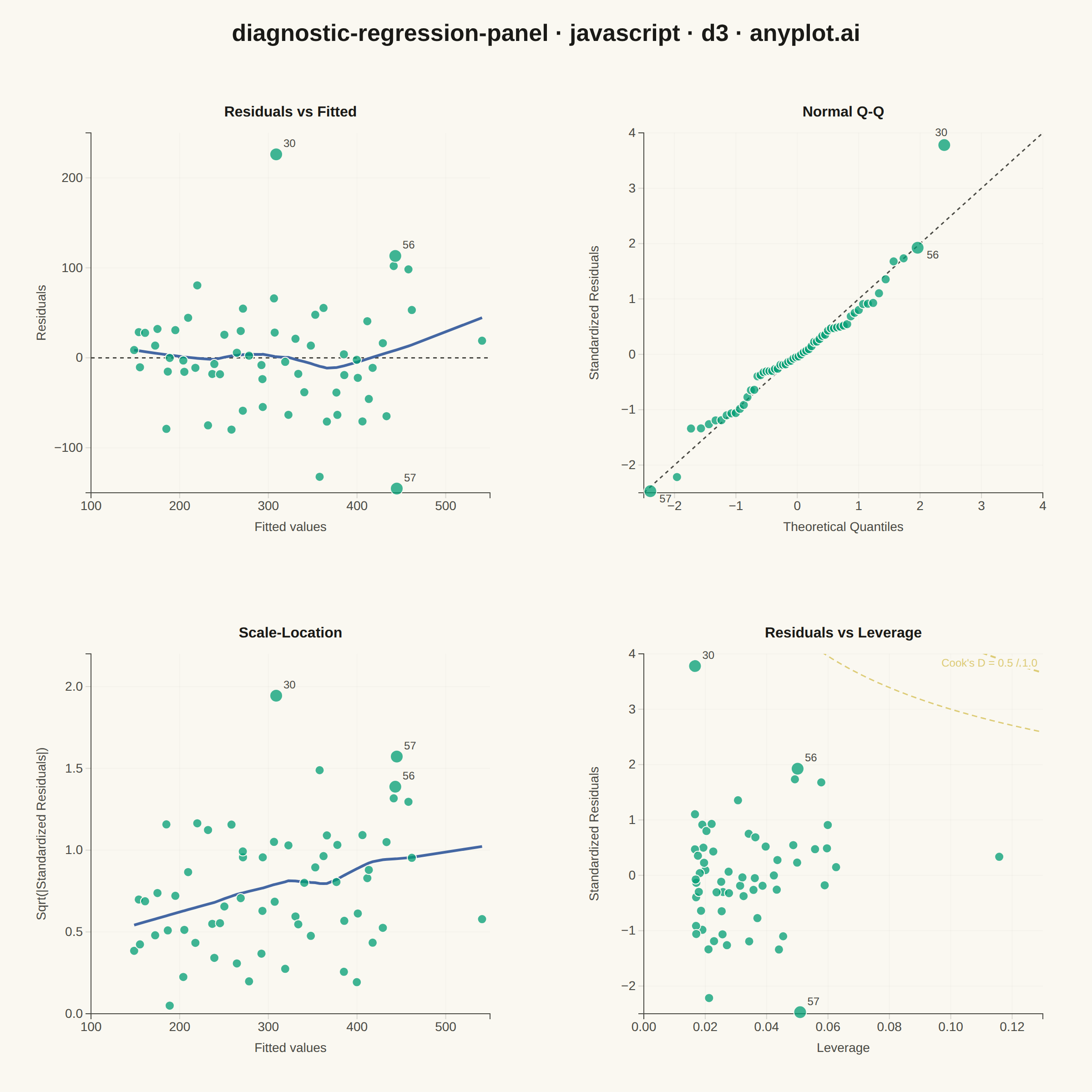
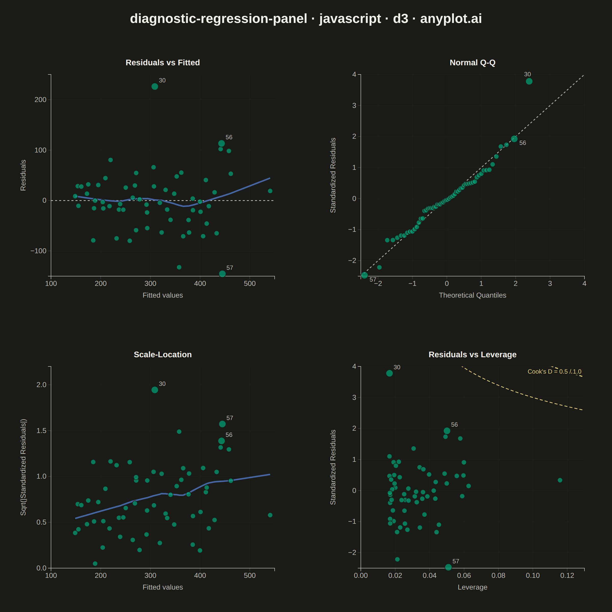
A 2x2 panel of diagnostic plots for evaluating linear regression model assumptions, replicating the classic output of R's `plot(lm)`. The four subplots are: (1) Residuals vs Fitted values to detect non-linearity and heteroscedasticity, (2) Normal Q-Q plot of standardized residuals to assess normality, (3) Scale-Location plot (square root of standardized residuals vs fitted values) to check homoscedasticity, and (4) Residuals vs Leverage with Cook's distance contours to identify influential observations. This composite display is the standard first step in regression model validation across statistics, academia, and regulated industries.
// anyplot.ai
// diagnostic-regression-panel: Regression Diagnostic Panel (Four-Plot Display)
// Library: d3 7.9.0 | JavaScript 22.23.2
// Quality: 88/100 | Updated: 2026-09-05
//# anyplot-orientation: square

const t = window.ANYPLOT_TOKENS;
const { width, height } = window.ANYPLOT_SIZE;

// --- Deterministic PRNG (LCG) + Box-Muller normal samples -------------------
let seed = 42;
function rand() {
  seed = (seed * 1664525 + 1013904223) % 4294967296;
  return seed / 4294967296;
}
function randNormal() {
  const u1 = Math.max(rand(), 1e-9);
  const u2 = rand();
  return Math.sqrt(-2 * Math.log(u1)) * Math.cos(2 * Math.PI * u2);
}

// --- Data: simple linear regression of home price on square footage --------
const n = 60;
const sqft = [];
const price = [];
for (let i = 0; i < n; i++) {
  const s = 800 + (i / (n - 1)) * 2700 + randNormal() * 40;
  const heteroNoise = randNormal() * (8 + s * 0.02); // variance grows with size
  sqft.push(s);
  price.push(50 + 0.12 * s + heteroNoise);
}
// inject a high-leverage point and two large-residual outliers
sqft[5] = 4200;
price[5] = 560;
price[30] += 140;
price[45] -= 130;

// --- OLS fit (simple linear regression) -------------------------------------
const xbar = d3.mean(sqft);
const ybar = d3.mean(price);
const Sxx = d3.sum(sqft.map((x) => (x - xbar) ** 2));
const Sxy = d3.sum(sqft.map((x, i) => (x - xbar) * (price[i] - ybar)));
const b1 = Sxy / Sxx;
const b0 = ybar - b1 * xbar;

const fitted = sqft.map((x) => b0 + b1 * x);
const residuals = price.map((y, i) => y - fitted[i]);
const p = 2; // parameters: intercept + slope
const rss = d3.sum(residuals.map((r) => r ** 2));
const sigma2 = rss / (n - p);
const leverage = sqft.map((x) => 1 / n + (x - xbar) ** 2 / Sxx);
const stdResid = residuals.map((r, i) => r / Math.sqrt(sigma2 * (1 - leverage[i])));
const sqrtAbsStdResid = stdResid.map((r) => Math.sqrt(Math.abs(r)));
const cooksD = stdResid.map((r, i) => (r ** 2 * leverage[i]) / (p * (1 - leverage[i])));

// three most influential observations by Cook's distance
const topInfluential = d3.range(n).sort((a, b) => cooksD[b] - cooksD[a]).slice(0, 3);

// --- Inverse normal CDF (Acklam's rational approximation) ------------------
function probit(pr) {
  const a = [-3.969683028665376e1, 2.209460984245205e2, -2.759285104469687e2,
    1.38357751867269e2, -3.066479806614716e1, 2.506628277459239];
  const b = [-5.447609879822406e1, 1.615858368580409e2, -1.556989798598866e2,
    6.680131188771972e1, -1.328068155288572e1];
  const c = [-7.784894002430293e-3, -3.223964580411365e-1, -2.400758277161838,
    -2.549732539343734, 4.374664141464968, 2.938163982698783];
  const d = [7.784695709041462e-3, 3.224671290700398e-1, 2.445134137142996, 3.754408661907416];
  const pLow = 0.02425;
  if (pr < pLow) {
    const q = Math.sqrt(-2 * Math.log(pr));
    return (((((c[0] * q + c[1]) * q + c[2]) * q + c[3]) * q + c[4]) * q + c[5]) /
      ((((d[0] * q + d[1]) * q + d[2]) * q + d[3]) * q + 1);
  }
  if (pr <= 1 - pLow) {
    const q = pr - 0.5;
    const r = q * q;
    return (((((a[0] * r + a[1]) * r + a[2]) * r + a[3]) * r + a[4]) * r + a[5]) * q /
      (((((b[0] * r + b[1]) * r + b[2]) * r + b[3]) * r + b[4]) * r + 1);
  }
  const q = Math.sqrt(-2 * Math.log(1 - pr));
  return -(((((c[0] * q + c[1]) * q + c[2]) * q + c[3]) * q + c[4]) * q + c[5]) /
    ((((d[0] * q + d[1]) * q + d[2]) * q + d[3]) * q + 1);
}

const qqOrder = d3.range(n).sort((i, j) => stdResid[i] - stdResid[j]);
const qqData = qqOrder.map((idx, rank) => ({
  theoretical: probit((rank + 0.5) / n),
  sample: stdResid[idx],
  idx,
}));

// --- LOWESS smoother (local linear regression, tricube weights) ------------
function lowess(xs, ys, frac) {
  const m = xs.length;
  const k = Math.max(2, Math.round(frac * m));
  const order = d3.range(m).sort((i, j) => xs[i] - xs[j]);
  const sx = order.map((i) => xs[i]);
  const sy = order.map((i) => ys[i]);
  return order.map((_, i) => {
    const dists = sx.map((x) => Math.abs(x - sx[i]));
    const bw = [...dists].sort((a, b) => a - b)[k - 1] || 1e-9;
    const weights = dists.map((dd) => (dd < bw ? (1 - (dd / bw) ** 3) ** 3 : 0));
    let sw = 0, swx = 0, swy = 0, swxx = 0, swxy = 0;
    for (let j = 0; j < m; j++) {
      const w = weights[j];
      sw += w; swx += w * sx[j]; swy += w * sy[j];
      swxx += w * sx[j] * sx[j]; swxy += w * sx[j] * sy[j];
    }
    const denom = sw * swxx - swx * swx;
    const intercept = Math.abs(denom) < 1e-9 ? swy / sw : (swy - ((sw * swxy - swx * swy) / denom) * swx) / sw;
    const slope = Math.abs(denom) < 1e-9 ? 0 : (sw * swxy - swx * swy) / denom;
    return { x: sx[i], y: intercept + slope * sx[i] };
  });
}

// --- Layout -------------------------------------------------------------
const svg = d3.select("#container").append("svg").attr("width", width).attr("height", height);
svg.append("rect").attr("width", width).attr("height", height).attr("fill", t.pageBg);

const titleH = 70;
const gutterX = 75;
const gutterY = 75;
const outer = 30;
const gridW = width - 2 * outer;
const gridH = height - titleH - 2 * outer;
const panelW = (gridW - gutterX) / 2;
const panelH = (gridH - gutterY) / 2;
const panelMargin = { top: 46, right: 24, bottom: 56, left: 70 };

svg.append("text")
  .attr("x", width / 2).attr("y", titleH / 2 + 10)
  .attr("text-anchor", "middle").attr("fill", t.ink)
  .style("font-size", "26px").style("font-weight", "600")
  .text("diagnostic-regression-panel · javascript · d3 · anyplot.ai");

const panelPositions = [
  { x0: outer, y0: outer + titleH },
  { x0: outer + panelW + gutterX, y0: outer + titleH },
  { x0: outer, y0: outer + titleH + panelH + gutterY },
  { x0: outer + panelW + gutterX, y0: outer + titleH + panelH + gutterY },
];

function styleAxis(sel) {
  sel.selectAll("text").attr("fill", t.inkSoft).style("font-size", "14px");
  sel.selectAll("line").attr("stroke", t.grid);
  sel.select(".domain").attr("stroke", t.inkSoft);
}

function panelChrome(g, iw, ih, title, xLabel, yLabel) {
  g.append("text").attr("x", iw / 2).attr("y", -18).attr("text-anchor", "middle")
    .attr("fill", t.ink).style("font-size", "16px").style("font-weight", "600").text(title);
  g.append("text").attr("x", iw / 2).attr("y", ih + 42).attr("text-anchor", "middle")
    .attr("fill", t.inkSoft).style("font-size", "14px").text(xLabel);
  g.append("text").attr("x", -ih / 2).attr("y", -50).attr("transform", "rotate(-90)")
    .attr("text-anchor", "middle").attr("fill", t.inkSoft).style("font-size", "14px").text(yLabel);
}

function addGrid(g, x, y, iw, ih) {
  g.append("g").selectAll("line.grid-y").data(y.ticks(5)).join("line")
    .attr("x1", 0).attr("x2", iw).attr("y1", (d) => y(d)).attr("y2", (d) => y(d))
    .attr("stroke", t.grid).attr("stroke-opacity", 0.15);
  g.append("g").selectAll("line.grid-x").data(x.ticks(5)).join("line")
    .attr("y1", 0).attr("y2", ih).attr("x1", (d) => x(d)).attr("x2", (d) => x(d))
    .attr("stroke", t.grid).attr("stroke-opacity", 0.15);
}

function labelInfluential(g, xs, ys, indices, offsetFn) {
  indices.forEach((i) => {
    const [dx, dy] = offsetFn ? offsetFn(i) : [8, -8];
    g.append("text").attr("x", xs(i) + dx).attr("y", ys(i) + dy)
      .attr("fill", t.inkSoft).style("font-size", "12px").text(i);
  });
}

// --- Panel 1: Residuals vs Fitted -------------------------------------------
{
  const pos = panelPositions[0];
  const g = svg.append("g").attr("transform", `translate(${pos.x0 + panelMargin.left},${pos.y0 + panelMargin.top})`);
  const iw = panelW - panelMargin.left - panelMargin.right;
  const ih = panelH - panelMargin.top - panelMargin.bottom;

  const x = d3.scaleLinear().domain(d3.extent(fitted)).nice().range([0, iw]);
  const y = d3.scaleLinear().domain(d3.extent(residuals)).nice().range([ih, 0]);

  addGrid(g, x, y, iw, ih);
  styleAxis(g.append("g").attr("transform", `translate(0,${ih})`).call(d3.axisBottom(x).ticks(5)));
  styleAxis(g.append("g").call(d3.axisLeft(y).ticks(5)));

  g.append("line").attr("x1", 0).attr("x2", iw).attr("y1", y(0)).attr("y2", y(0))
    .attr("stroke", t.inkSoft).attr("stroke-dasharray", "4,4").attr("stroke-width", 1.5);

  const smooth = lowess(fitted, residuals, 0.6);
  const line = d3.line().x((d) => x(d.x)).y((d) => y(d.y));
  g.append("path").datum(smooth).attr("d", line).attr("fill", "none")
    .attr("stroke", t.palette[2]).attr("stroke-width", 3);

  g.selectAll("circle").data(d3.range(n)).join("circle")
    .attr("cx", (i) => x(fitted[i])).attr("cy", (i) => y(residuals[i]))
    .attr("r", (i) => (topInfluential.includes(i) ? 7 : 5))
    .attr("fill", t.palette[0]).attr("fill-opacity", 0.75)
    .attr("stroke", t.pageBg).attr("stroke-width", 1);

  labelInfluential(g, (i) => x(fitted[i]), (i) => y(residuals[i]), topInfluential);
  panelChrome(g, iw, ih, "Residuals vs Fitted", "Fitted values", "Residuals");
}

// --- Panel 2: Normal Q-Q -----------------------------------------------------
{
  const pos = panelPositions[1];
  const g = svg.append("g").attr("transform", `translate(${pos.x0 + panelMargin.left},${pos.y0 + panelMargin.top})`);
  const iw = panelW - panelMargin.left - panelMargin.right;
  const ih = panelH - panelMargin.top - panelMargin.bottom;

  const domain = d3.extent([...qqData.map((d) => d.theoretical), ...qqData.map((d) => d.sample)]);
  const x = d3.scaleLinear().domain(domain).nice().range([0, iw]);
  const y = d3.scaleLinear().domain(domain).nice().range([ih, 0]);

  addGrid(g, x, y, iw, ih);
  styleAxis(g.append("g").attr("transform", `translate(0,${ih})`).call(d3.axisBottom(x).ticks(5)));
  styleAxis(g.append("g").call(d3.axisLeft(y).ticks(5)));

  const refDomain = x.domain();
  g.append("line")
    .attr("x1", x(refDomain[0])).attr("y1", y(refDomain[0]))
    .attr("x2", x(refDomain[1])).attr("y2", y(refDomain[1]))
    .attr("stroke", t.inkSoft).attr("stroke-dasharray", "4,4").attr("stroke-width", 1.5);

  g.selectAll("circle").data(qqData).join("circle")
    .attr("cx", (d) => x(d.theoretical)).attr("cy", (d) => y(d.sample))
    .attr("r", (d) => (topInfluential.includes(d.idx) ? 7 : 5))
    .attr("fill", t.palette[0]).attr("fill-opacity", 0.75)
    .attr("stroke", t.pageBg).attr("stroke-width", 1);

  const byIdx = new Map(qqData.map((d) => [d.idx, d]));
  // The 45-degree reference line runs bottom-left to top-right on screen; a
  // (+8,-8) offset moves roughly parallel to it, which is why labels used to
  // merge with the line. Offset perpendicular instead, direction chosen by
  // which side of the line the point actually falls on.
  labelInfluential(
    g,
    (i) => x(byIdx.get(i).theoretical),
    (i) => y(byIdx.get(i).sample),
    topInfluential,
    (i) => {
      const d = byIdx.get(i);
      const aboveLine = y(d.sample) < y(d.theoretical);
      return aboveLine ? [-10, -10] : [10, 12];
    },
  );
  panelChrome(g, iw, ih, "Normal Q-Q", "Theoretical Quantiles", "Standardized Residuals");
}

// --- Panel 3: Scale-Location --------------------------------------------------
{
  const pos = panelPositions[2];
  const g = svg.append("g").attr("transform", `translate(${pos.x0 + panelMargin.left},${pos.y0 + panelMargin.top})`);
  const iw = panelW - panelMargin.left - panelMargin.right;
  const ih = panelH - panelMargin.top - panelMargin.bottom;

  const x = d3.scaleLinear().domain(d3.extent(fitted)).nice().range([0, iw]);
  const y = d3.scaleLinear().domain([0, d3.max(sqrtAbsStdResid) * 1.1]).nice().range([ih, 0]);

  addGrid(g, x, y, iw, ih);
  styleAxis(g.append("g").attr("transform", `translate(0,${ih})`).call(d3.axisBottom(x).ticks(5)));
  styleAxis(g.append("g").call(d3.axisLeft(y).ticks(5)));

  const smooth = lowess(fitted, sqrtAbsStdResid, 0.6);
  const line = d3.line().x((d) => x(d.x)).y((d) => y(d.y));
  g.append("path").datum(smooth).attr("d", line).attr("fill", "none")
    .attr("stroke", t.palette[2]).attr("stroke-width", 3);

  g.selectAll("circle").data(d3.range(n)).join("circle")
    .attr("cx", (i) => x(fitted[i])).attr("cy", (i) => y(sqrtAbsStdResid[i]))
    .attr("r", (i) => (topInfluential.includes(i) ? 7 : 5))
    .attr("fill", t.palette[0]).attr("fill-opacity", 0.75)
    .attr("stroke", t.pageBg).attr("stroke-width", 1);

  labelInfluential(g, (i) => x(fitted[i]), (i) => y(sqrtAbsStdResid[i]), topInfluential);
  panelChrome(g, iw, ih, "Scale-Location", "Fitted values", "Sqrt(|Standardized Residuals|)");
}

// --- Panel 4: Residuals vs Leverage (with Cook's distance contours) --------
{
  const pos = panelPositions[3];
  const g = svg.append("g").attr("transform", `translate(${pos.x0 + panelMargin.left},${pos.y0 + panelMargin.top})`);
  const iw = panelW - panelMargin.left - panelMargin.right;
  const ih = panelH - panelMargin.top - panelMargin.bottom;

  const x = d3.scaleLinear().domain([0, d3.max(leverage) * 1.1]).nice().range([0, iw]);
  const y = d3.scaleLinear().domain(d3.extent(stdResid)).nice().range([ih, 0]);

  addGrid(g, x, y, iw, ih);
  styleAxis(g.append("g").attr("transform", `translate(0,${ih})`).call(d3.axisBottom(x).ticks(5)));
  styleAxis(g.append("g").call(d3.axisLeft(y).ticks(5)));

  g.append("clipPath").attr("id", "clip-leverage").append("rect").attr("width", iw).attr("height", ih);

  const hMax = x.domain()[1];
  const hGrid = d3.range(1, 200).map((i) => (i / 200) * hMax);
  const contourLine = d3.line().x((d) => x(d.h)).y((d) => y(d.val));
  [
    { D: 0.5, width: 1.5 },
    { D: 1.0, width: 2 },
  ].forEach(({ D, width: lw }) => {
    const upper = hGrid.map((h) => ({ h, val: Math.sqrt((D * p * (1 - h)) / h) }));
    const lower = upper.map((d) => ({ h: d.h, val: -d.val }));
    [upper, lower].forEach((series) => {
      g.append("path").attr("clip-path", "url(#clip-leverage)").datum(series).attr("d", contourLine)
        .attr("fill", "none").attr("stroke", t.amber).attr("stroke-width", lw).attr("stroke-dasharray", "6,4");
    });
  });

  g.selectAll("circle").data(d3.range(n)).join("circle")
    .attr("cx", (i) => x(leverage[i])).attr("cy", (i) => y(stdResid[i]))
    .attr("r", (i) => (topInfluential.includes(i) ? 7 : 5))
    .attr("fill", t.palette[0]).attr("fill-opacity", 0.75)
    .attr("stroke", t.pageBg).attr("stroke-width", 1);

  labelInfluential(g, (i) => x(leverage[i]), (i) => y(stdResid[i]), topInfluential);
  panelChrome(g, iw, ih, "Residuals vs Leverage", "Leverage", "Standardized Residuals");

  g.append("text").attr("x", iw - 6).attr("y", 14).attr("text-anchor", "end")
    .attr("fill", t.amber).style("font-size", "12px")
    .style("paint-order", "stroke").attr("stroke", t.pageBg).attr("stroke-width", 5).attr("stroke-linejoin", "round")
    .text("Cook's D = 0.5 / 1.0");
}
Runnable source as JSON, for any HTTP client: https://api.anyplot.ai/specs/diagnostic-regression-panel/d3/code. Any spec id and library id listed in llms-full.txt fit the same URL shape; every URL below is complete and callable.
{
  "spec_id": "diagnostic-regression-panel",
  "language": "javascript",
  "library": "d3",
  "page": "https://anyplot.ai/diagnostic-regression-panel/javascript/d3",
  "hub": "https://anyplot.ai/diagnostic-regression-panel",
  "code_json": "https://api.anyplot.ai/specs/diagnostic-regression-panel/d3/code",
  "spec_json": "https://api.anyplot.ai/specs/diagnostic-regression-panel",
  "render_light_png": "https://storage.googleapis.com/anyplot-images/plots/diagnostic-regression-panel/javascript/d3/plot-light.png",
  "render_dark_png": "https://storage.googleapis.com/anyplot-images/plots/diagnostic-regression-panel/javascript/d3/plot-dark.png",
  "interactive_light_html": "https://storage.googleapis.com/anyplot-images/plots/diagnostic-regression-panel/javascript/d3/plot-light.html",
  "interactive_dark_html": "https://storage.googleapis.com/anyplot-images/plots/diagnostic-regression-panel/javascript/d3/plot-dark.html",
  "quality_score": 88.0,
  "license": "MIT",
  "guide": "https://anyplot.ai/llms.txt"
}
Part of Regression Diagnostic Panel (Four-Plot Display) on anyplot.ai.