The same plot in 14 other libraries — Python: Altair, Bokeh, lets-plot, Plotly, plotnine, Pygal, Seaborn; R: ggplot2; Julia: Makie.jl; JavaScript: Chart.js, D3.js, Apache ECharts, Highcharts, MUI X Charts. Compare all 15 side by side: Regression Diagnostic Panel (Four-Plot Display) in Python, R, Julia and JavaScript.
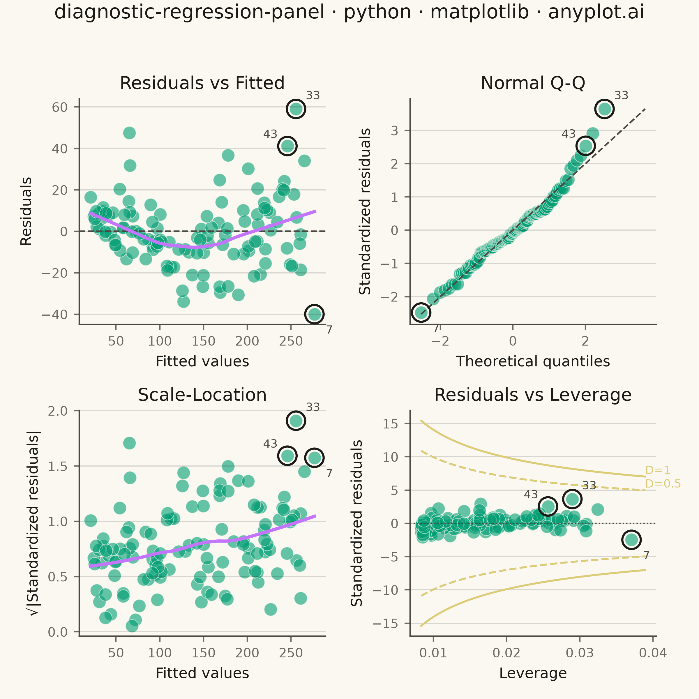
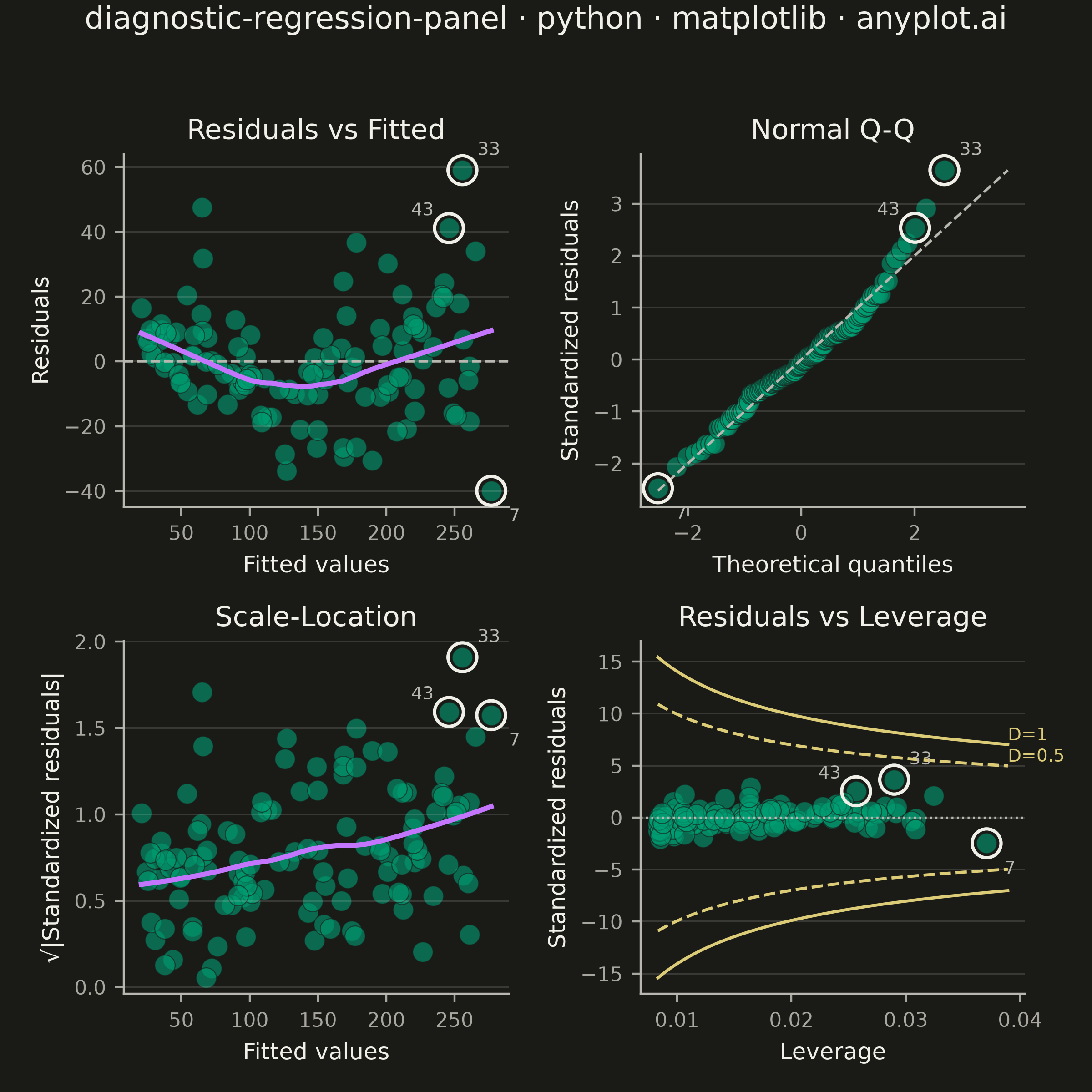
A 2x2 panel of diagnostic plots for evaluating linear regression model assumptions, replicating the classic output of R's `plot(lm)`. The four subplots are: (1) Residuals vs Fitted values to detect non-linearity and heteroscedasticity, (2) Normal Q-Q plot of standardized residuals to assess normality, (3) Scale-Location plot (square root of standardized residuals vs fitted values) to check homoscedasticity, and (4) Residuals vs Leverage with Cook's distance contours to identify influential observations. This composite display is the standard first step in regression model validation across statistics, academia, and regulated industries.
""" anyplot.ai
diagnostic-regression-panel: Regression Diagnostic Panel (Four-Plot Display)
Library: matplotlib 3.11.1 | Python 3.13.15
Quality: 90/100 | Created: 2026-08-24
"""

import os

import matplotlib.pyplot as plt
import numpy as np
import statsmodels.api as sm
from scipy import stats


# Theme tokens (see prompts/default-style-guide.md "Background" + "Theme-adaptive Chrome")
THEME = os.getenv("ANYPLOT_THEME", "light")
PAGE_BG = "#FAF8F1" if THEME == "light" else "#1A1A17"
INK = "#1A1A17" if THEME == "light" else "#F0EFE8"
INK_SOFT = "#4A4A44" if THEME == "light" else "#B8B7B0"
INK_MUTED = "#6B6A63" if THEME == "light" else "#A8A79F"

# Imprint palette — position 1 is always brand green
BRAND = "#009E73"
LOWESS_COLOR = "#C475FD"  # Imprint palette position 2
AMBER = "#DDCC77"  # semantic anchor — Cook's distance warning contours

# Data: fit an OLS dose-response model on heteroscedastic, mildly non-linear data
np.random.seed(42)
n = 120
dose_mg = np.random.uniform(5, 95, n)
noise_scale = 1.0 + 0.035 * dose_mg
response = 22 + 1.65 * dose_mg + 0.012 * dose_mg**2 + np.random.normal(0, 5, n) * noise_scale

# A few deliberately influential observations (high leverage / high residual)
response[3] += 55
response[15] += 48
dose_mg[7] = 98

design_matrix = sm.add_constant(dose_mg)
model = sm.OLS(response, design_matrix).fit()
influence = model.get_influence()

fitted = model.fittedvalues
resid = model.resid
std_resid = influence.resid_studentized_internal
leverage = influence.hat_matrix_diag
cooks_d = influence.cooks_distance[0]
n_params = design_matrix.shape[1]

top_influential = np.argsort(cooks_d)[-3:][::-1]

# Plot — 2x2 diagnostic grid, square canvas since the layout is grid-based/symmetric
fig, axes = plt.subplots(2, 2, figsize=(6, 6), dpi=400, facecolor=PAGE_BG)
for panel in axes.flat:
    panel.set_facecolor(PAGE_BG)

point_kw = {"s": 65, "color": BRAND, "alpha": 0.6, "edgecolors": PAGE_BG, "linewidth": 0.4}
highlight_kw = {"s": 130, "facecolors": "none", "edgecolors": INK, "linewidth": 1.3, "zorder": 5}
label_kw = {"fontsize": 7, "color": INK_SOFT, "textcoords": "offset points"}
# Distinct offset per influential point (same point keeps the same offset in every
# subplot) so the three labels fan out instead of clustering together.
label_offsets = [(6, 6), (7, -12), (-15, 5)]

# Subplot 1: Residuals vs Fitted
ax = axes[0, 0]
ax.scatter(fitted, resid, **point_kw)
ax.scatter(fitted[top_influential], resid[top_influential], **highlight_kw)
ax.axhline(0, color=INK_SOFT, linewidth=1.0, linestyle="--")
lowess_rf = sm.nonparametric.lowess(resid, fitted, frac=0.6)
ax.plot(lowess_rf[:, 0], lowess_rf[:, 1], color=LOWESS_COLOR, linewidth=2.0)
for i, idx in enumerate(top_influential):
    ax.annotate(str(idx), (fitted[idx], resid[idx]), xytext=label_offsets[i], **label_kw)
ax.set_title("Residuals vs Fitted", fontsize=11, color=INK)
ax.set_xlabel("Fitted values", fontsize=9, color=INK)
ax.set_ylabel("Residuals", fontsize=9, color=INK)

# Subplot 2: Normal Q-Q
ax = axes[0, 1]
osm, osr = stats.probplot(std_resid, dist="norm", fit=False)
ax.scatter(osm, osr, **point_kw)
qq_bound = (min(osm.min(), osr.min()), max(osm.max(), osr.max()))
ax.plot(qq_bound, qq_bound, color=INK_SOFT, linewidth=1.0, linestyle="--")
sorted_idx = np.argsort(std_resid)
rank_of = {obs: rank for rank, obs in enumerate(sorted_idx)}
qq_influential_x = [osm[rank_of[idx]] for idx in top_influential]
qq_influential_y = [osr[rank_of[idx]] for idx in top_influential]
ax.scatter(qq_influential_x, qq_influential_y, **highlight_kw)
for i, idx in enumerate(top_influential):
    ax.annotate(str(idx), (osm[rank_of[idx]], osr[rank_of[idx]]), xytext=label_offsets[i], **label_kw)
ax.set_title("Normal Q-Q", fontsize=11, color=INK)
ax.set_xlabel("Theoretical quantiles", fontsize=9, color=INK)
ax.set_ylabel("Standardized residuals", fontsize=9, color=INK)

# Subplot 3: Scale-Location
ax = axes[1, 0]
sqrt_std_resid = np.sqrt(np.abs(std_resid))
ax.scatter(fitted, sqrt_std_resid, **point_kw)
ax.scatter(fitted[top_influential], sqrt_std_resid[top_influential], **highlight_kw)
lowess_sl = sm.nonparametric.lowess(sqrt_std_resid, fitted, frac=0.6)
ax.plot(lowess_sl[:, 0], lowess_sl[:, 1], color=LOWESS_COLOR, linewidth=2.0)
for i, idx in enumerate(top_influential):
    ax.annotate(str(idx), (fitted[idx], sqrt_std_resid[idx]), xytext=label_offsets[i], **label_kw)
ax.set_title("Scale-Location", fontsize=11, color=INK)
ax.set_xlabel("Fitted values", fontsize=9, color=INK)
ax.set_ylabel("√|Standardized residuals|", fontsize=9, color=INK)

# Subplot 4: Residuals vs Leverage with Cook's distance contours
ax = axes[1, 1]
ax.scatter(leverage, std_resid, **point_kw)
ax.scatter(leverage[top_influential], std_resid[top_influential], **highlight_kw)
ax.axhline(0, color=INK_SOFT, linewidth=0.8, linestyle=":")
h_grid = np.linspace(max(leverage.min(), 1e-3), leverage.max() * 1.05, 200)
for cooks_level, style in ((0.5, "--"), (1.0, "-")):
    bound = np.sqrt(cooks_level * n_params * (1 - h_grid) / h_grid)
    ax.plot(h_grid, bound, color=AMBER, linewidth=1.2, linestyle=style)
    ax.plot(h_grid, -bound, color=AMBER, linewidth=1.2, linestyle=style)
    ax.text(h_grid[-1], bound[-1], f"D={cooks_level:g}", fontsize=7, color=AMBER, va="bottom")
for i, idx in enumerate(top_influential):
    ax.annotate(str(idx), (leverage[idx], std_resid[idx]), xytext=label_offsets[i], **label_kw)
ax.set_title("Residuals vs Leverage", fontsize=11, color=INK)
ax.set_xlabel("Leverage", fontsize=9, color=INK)
ax.set_ylabel("Standardized residuals", fontsize=9, color=INK)

# Shared chrome across all four subplots
for panel in axes.flat:
    panel.tick_params(axis="both", labelsize=8, colors=INK_MUTED, labelcolor=INK_MUTED)
    panel.spines["top"].set_visible(False)
    panel.spines["right"].set_visible(False)
    for side in ("left", "bottom"):
        panel.spines[side].set_color(INK_SOFT)
    panel.yaxis.grid(True, alpha=0.15, linewidth=0.7, color=INK)

title = "diagnostic-regression-panel · python · matplotlib · anyplot.ai"
title_fontsize = 12 if len(title) <= 67 else max(8, round(12 * 67 / len(title)))
fig.suptitle(title, fontsize=title_fontsize, fontweight="medium", color=INK, y=0.995)

# Save
fig.tight_layout(rect=(0, 0, 1, 0.97))
plt.savefig(f"plot-{THEME}.png", dpi=400, facecolor=PAGE_BG)  # bbox_inches MUST stay default
Runnable source as JSON, for any HTTP client: https://api.anyplot.ai/specs/diagnostic-regression-panel/matplotlib/code. Any spec id and library id listed in llms-full.txt fit the same URL shape; every URL below is complete and callable.
{
  "spec_id": "diagnostic-regression-panel",
  "language": "python",
  "library": "matplotlib",
  "page": "https://anyplot.ai/diagnostic-regression-panel/python/matplotlib",
  "hub": "https://anyplot.ai/diagnostic-regression-panel",
  "code_json": "https://api.anyplot.ai/specs/diagnostic-regression-panel/matplotlib/code",
  "spec_json": "https://api.anyplot.ai/specs/diagnostic-regression-panel",
  "render_light_png": "https://storage.googleapis.com/anyplot-images/plots/diagnostic-regression-panel/python/matplotlib/plot-light.png",
  "render_dark_png": "https://storage.googleapis.com/anyplot-images/plots/diagnostic-regression-panel/python/matplotlib/plot-dark.png",
  "quality_score": 90.0,
  "license": "MIT",
  "guide": "https://anyplot.ai/llms.txt"
}
Part of Regression Diagnostic Panel (Four-Plot Display) on anyplot.ai.