The same plot in 14 other libraries — JavaScript: Chart.js, D3.js, Apache ECharts, Highcharts; Python: Altair, Bokeh, lets-plot, Matplotlib, Plotly, plotnine, Pygal, Seaborn; R: ggplot2; Julia: Makie.jl. Compare all 15 side by side: Regression Diagnostic Panel (Four-Plot Display) in Python, R, Julia and JavaScript.
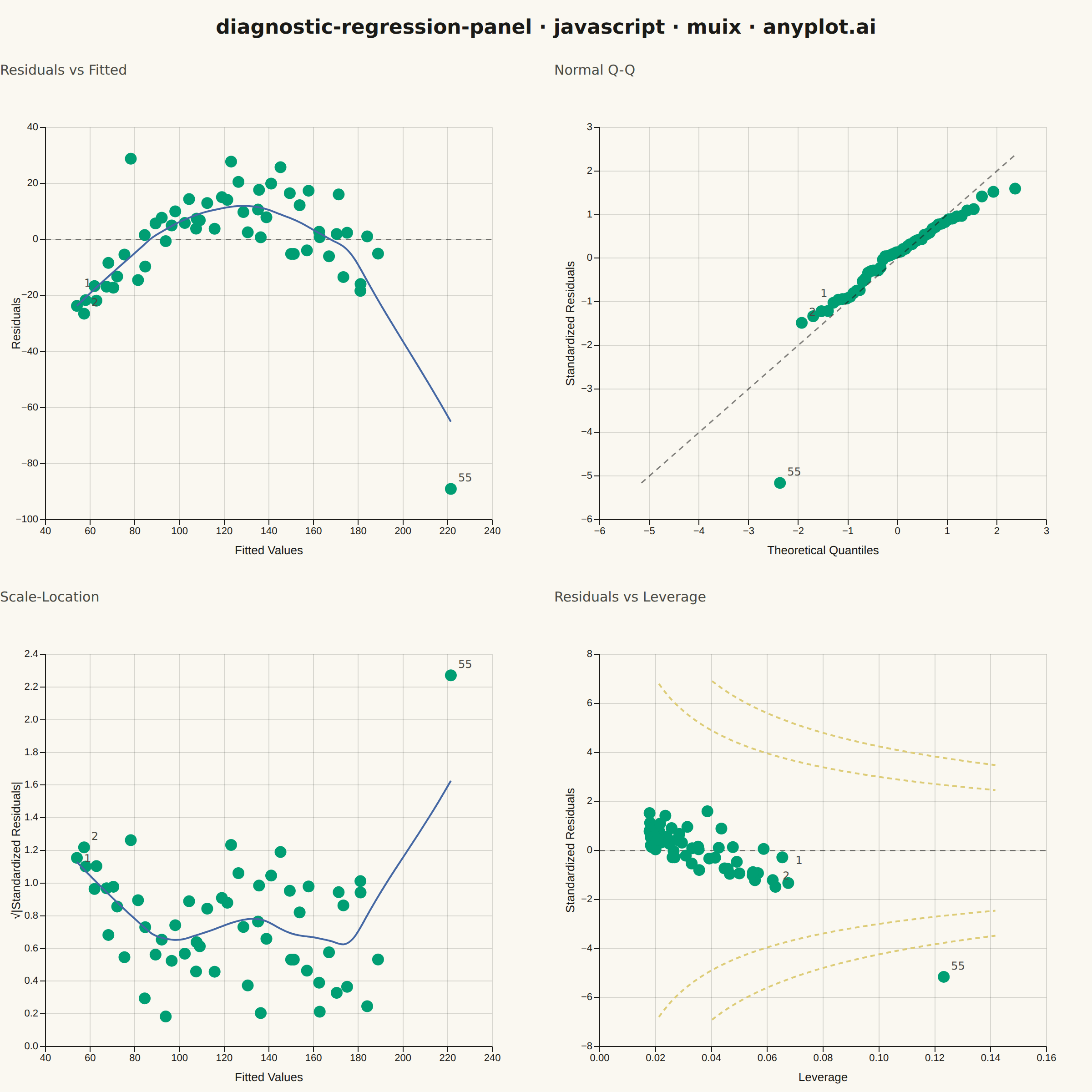
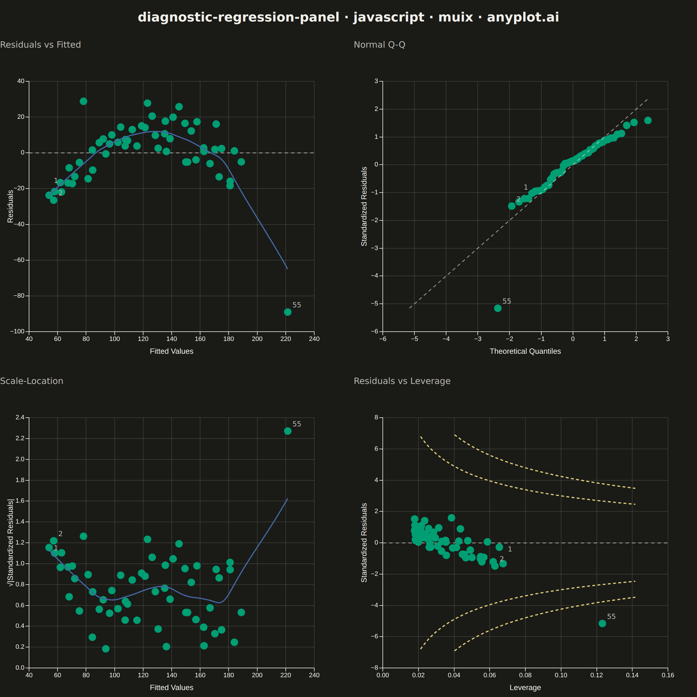
A 2x2 panel of diagnostic plots for evaluating linear regression model assumptions, replicating the classic output of R's `plot(lm)`. The four subplots are: (1) Residuals vs Fitted values to detect non-linearity and heteroscedasticity, (2) Normal Q-Q plot of standardized residuals to assess normality, (3) Scale-Location plot (square root of standardized residuals vs fitted values) to check homoscedasticity, and (4) Residuals vs Leverage with Cook's distance contours to identify influential observations. This composite display is the standard first step in regression model validation across statistics, academia, and regulated industries.
// anyplot.ai
// diagnostic-regression-panel: Regression Diagnostic Panel (Four-Plot Display)
// Library: muix 7.29.1 | JavaScript 22.23.2
// Quality: 90/100 | Created: 2026-09-05
//# anyplot-orientation: square
// anyplot.ai
// diagnostic-regression-panel: Regression Diagnostic Panel (Four-Plot Display)
// Library: MUI X Charts | React | Node 22
// License: @mui/x-charts — MIT (community). Pro/Premium are out of scope.
// Quality: pending | Created: 2026-09-05
import * as React from "react";
import { ChartContainer } from "@mui/x-charts/ChartContainer";
import { ScatterPlot } from "@mui/x-charts/ScatterChart";
import { LinePlot } from "@mui/x-charts/LineChart";
import { ChartsXAxis } from "@mui/x-charts/ChartsXAxis";
import { ChartsYAxis } from "@mui/x-charts/ChartsYAxis";
import { ChartsGrid } from "@mui/x-charts/ChartsGrid";
import { ChartsReferenceLine } from "@mui/x-charts/ChartsReferenceLine";
import { ChartsText } from "@mui/x-charts/ChartsText";
import { useXScale, useYScale } from "@mui/x-charts/hooks";

const t = window.ANYPLOT_TOKENS;
const FONT = "system-ui, -apple-system, 'Segoe UI', sans-serif";

// --- Deterministic PRNG (LCG) + Box-Muller normal --------------------------
let seed = 20260905;
function nextUniform() {
  seed = (seed * 1103515245 + 12345) & 0x7fffffff;
  return seed / 0x7fffffff;
}
function nextNormal() {
  const u1 = Math.max(nextUniform(), 1e-9);
  const u2 = nextUniform();
  return Math.sqrt(-2 * Math.log(u1)) * Math.cos(2 * Math.PI * u2);
}

// --- Data: dose-response study (drug dose vs biomarker response) -----------
const N = 56;
const dose = [];
for (let i = 0; i < N; i++) {
  dose.push(4 + 92 * (i / (N - 1)) + (nextUniform() - 0.5) * 3);
}
dose.sort((a, b) => a - b);

const response = dose.map((d) => {
  const trend = 18 + 2.9 * d - 0.012 * d * d; // mild curvature
  const noiseScale = 2.5 + 0.11 * d; // heteroscedastic — variance grows with dose
  return trend + nextNormal() * noiseScale;
});

// Two deliberately influential observations, so the panel has something to diagnose
response[10] += 34; // large residual, moderate leverage
dose[N - 2] = 118;
response[N - 2] -= 46; // high leverage + large residual

// --- Ordinary least squares (simple linear regression) ---------------------
const n = dose.length;
const p = 2; // parameters: intercept + slope
const doseMean = dose.reduce((a, b) => a + b, 0) / n;
const responseMean = response.reduce((a, b) => a + b, 0) / n;
const sxx = dose.reduce((acc, d) => acc + (d - doseMean) ** 2, 0);
const sxy = dose.reduce((acc, d, i) => acc + (d - doseMean) * (response[i] - responseMean), 0);
const slope = sxy / sxx;
const intercept = responseMean - slope * doseMean;

const fitted = dose.map((d) => intercept + slope * d);
const residuals = response.map((y, i) => y - fitted[i]);
const rss = residuals.reduce((acc, r) => acc + r * r, 0);
const sigma = Math.sqrt(rss / (n - p));
const leverage = dose.map((d) => 1 / n + (d - doseMean) ** 2 / sxx);
const stdResiduals = residuals.map((r, i) => r / (sigma * Math.sqrt(1 - leverage[i])));
const scaleLocation = stdResiduals.map((r) => Math.sqrt(Math.abs(r)));
const cooksD = stdResiduals.map((r, i) => (r * r * leverage[i]) / (p * (1 - leverage[i])));

// Three most influential observations (highest Cook's distance), labeled by 1-based index
const influentialIdx = cooksD
  .map((d, i) => [d, i])
  .sort((a, b) => b[0] - a[0])
  .slice(0, 3)
  .map(([, i]) => i);

// --- Normal Q-Q: theoretical quantiles vs sorted standardized residuals ----
function inverseNormalCdf(pr) {
  // Acklam's rational approximation of the standard normal quantile function
  const a = [-3.969683028665376e1, 2.209460984245205e2, -2.759285104469687e2, 1.38357751867269e2, -3.066479806614716e1, 2.506628277459239];
  const b = [-5.447609879822406e1, 1.615858368580409e2, -1.556989798598866e2, 6.680131188771972e1, -1.328068155288572e1];
  const c = [-7.784894002430293e-3, -3.223964580411365e-1, -2.400758277161838, -2.549732539343734, 4.374664141464968, 2.938163982698783];
  const d = [7.784695709041462e-3, 3.224671290700398e-1, 2.445134137142996, 3.754408661907416];
  const low = 0.02425;
  if (pr < low) {
    const q = Math.sqrt(-2 * Math.log(pr));
    return (((((c[0] * q + c[1]) * q + c[2]) * q + c[3]) * q + c[4]) * q + c[5]) / ((((d[0] * q + d[1]) * q + d[2]) * q + d[3]) * q + 1);
  }
  if (pr > 1 - low) {
    const q = Math.sqrt(-2 * Math.log(1 - pr));
    return -(((((c[0] * q + c[1]) * q + c[2]) * q + c[3]) * q + c[4]) * q + c[5]) / ((((d[0] * q + d[1]) * q + d[2]) * q + d[3]) * q + 1);
  }
  const q = pr - 0.5;
  const r = q * q;
  return (((((a[0] * r + a[1]) * r + a[2]) * r + a[3]) * r + a[4]) * r + a[5]) * q / (((((b[0] * r + b[1]) * r + b[2]) * r + b[3]) * r + b[4]) * r + 1);
}

const qqRanked = stdResiduals.map((v, i) => [v, i]).sort((a, b) => a[0] - b[0]);
const theoreticalQuantiles = new Array(n);
const sortedStdResiduals = new Array(n);
const qqRankByOrigIdx = new Array(n);
qqRanked.forEach(([v, origIdx], rank) => {
  theoreticalQuantiles[rank] = inverseNormalCdf((rank + 0.5) / n);
  sortedStdResiduals[rank] = v;
  qqRankByOrigIdx[origIdx] = rank;
});

// --- LOWESS (locally weighted linear regression, tricube kernel) -----------
function linspace(min, max, count) {
  if (count <= 1) return [min];
  const step = (max - min) / (count - 1);
  return Array.from({ length: count }, (_, i) => min + step * i);
}

function lowess(xs, ys, xGrid, bandwidthFraction) {
  const m = xs.length;
  const k = Math.max(3, Math.round(bandwidthFraction * m));
  return xGrid.map((x0) => {
    const dists = xs.map((xi) => Math.abs(xi - x0));
    const bandwidth = [...dists].sort((a, b) => a - b)[Math.min(k - 1, m - 1)] || 1e-6;
    let sw = 0, swx = 0, swy = 0, swxx = 0, swxy = 0;
    for (let i = 0; i < m; i++) {
      const u = dists[i] / bandwidth;
      if (u >= 1) continue;
      const w = (1 - u ** 3) ** 3; // tricube weight
      sw += w; swx += w * xs[i]; swy += w * ys[i];
      swxx += w * xs[i] * xs[i]; swxy += w * xs[i] * ys[i];
    }
    const denom = sw * swxx - swx * swx;
    if (Math.abs(denom) < 1e-9) return swy / sw;
    const b1 = (sw * swxy - swx * swy) / denom;
    const b0 = (swy - b1 * swx) / sw;
    return b0 + b1 * x0;
  });
}

const fittedGrid = linspace(Math.min(...fitted), Math.max(...fitted), 36);
const residLowess = lowess(fitted, residuals, fittedGrid, 0.5);
const scaleLocLowess = lowess(fitted, scaleLocation, fittedGrid, 0.5);

// --- Q-Q reference line: y = x across the combined data range --------------
const qqMin = Math.min(...theoreticalQuantiles, ...sortedStdResiduals);
const qqMax = Math.max(...theoreticalQuantiles, ...sortedStdResiduals);
const qqDiagonalGrid = [qqMin, qqMax];

// --- Cook's distance contours (Residuals vs Leverage) -----------------------
const leverageMax = Math.max(...leverage);
const leverageGrid = linspace(Math.max(0.004, Math.min(...leverage) * 0.3), leverageMax * 1.15, 44);
const cookYCap = Math.max(3, Math.max(...stdResiduals.map(Math.abs)) * 1.35);
function cookBranch(cooksLevel) {
  return leverageGrid.map((h) => {
    const v = Math.sqrt((cooksLevel * p * (1 - h)) / h);
    return v > cookYCap ? null : v;
  });
}
const cookHalfPos = cookBranch(0.5);
const cookHalfNeg = cookHalfPos.map((v) => (v === null ? null : -v));
const cookOnePos = cookBranch(1.0);
const cookOneNeg = cookOnePos.map((v) => (v === null ? null : -v));

// --- Shared styling ----------------------------------------------------------
const POINT_COLOR = t.palette[0]; // brand green — same marker color in all four subplots
const SMOOTH_COLOR = t.palette[2]; // blue trend line
const CONTOUR_COLOR = t.amber; // warning/threshold semantic color for Cook's distance
const REF_LINE_STYLE = { stroke: t.ink, strokeWidth: 1.5, strokeDasharray: "6 5", opacity: 0.55 };
const CONTOUR_LINE_STYLE = { strokeDasharray: "5 4" };
const MARKER_SIZE = 6.5;
const AXIS_LABEL_STYLE = { fontSize: 13 };
const TICK_LABEL_STYLE = { fontSize: 11 };

function scatterSeries(id, xs, ys) {
  return {
    id,
    type: "scatter",
    color: POINT_COLOR,
    markerSize: MARKER_SIZE,
    data: xs.map((x, i) => ({ x, y: ys[i], id: i })),
  };
}

// Labels the top-3 most-influential observations inside a chart's SVG space.
// Must run as a child of ChartContainer to read the live x/y scales.
// Two labels whose marker centers are closer than this (Euclidean, px) are
// considered crowded and get staggered vertically so their index numbers
// don't visually merge — covers both stacked and side-by-side markers.
const LABEL_CROWD_PX = 20;
const LABEL_STAGGER_PX = 13;

function InfluentialLabels({ points }) {
  const xScale = useXScale();
  const yScale = useYScale();
  const positioned = points
    .map(({ x, y, text }) => {
      const px = xScale(x);
      const py = yScale(y);
      if (px == null || py == null || Number.isNaN(px) || Number.isNaN(py)) return null;
      return { px, py, text };
    })
    .filter(Boolean);

  // Stagger along the direction away from the colliding neighbor, so a point
  // below its neighbor moves further down (not toward it).
  positioned.forEach((point, i) => {
    let stackOffset = 0;
    let sign = 1;
    for (let j = 0; j < i; j++) {
      const other = positioned[j];
      const dist = Math.hypot(point.px - other.px, point.py - other.py);
      if (dist < LABEL_CROWD_PX) {
        stackOffset += 1;
        sign = point.py >= other.py ? -1 : 1;
      }
    }
    point.dy = sign * stackOffset * LABEL_STAGGER_PX;
  });

  return (
    <React.Fragment>
      {positioned.map(({ px, py, text, dy }) => (
        <ChartsText
          key={text}
          x={px + 8}
          y={py - 8 - dy}
          text={text}
          fill={t.inkSoft}
          style={{ fontSize: 12, fontFamily: FONT, textAnchor: "start" }}
        />
      ))}
    </React.Fragment>
  );
}

function SubplotTitle({ children, height }) {
  return (
    <div style={{ height, display: "flex", alignItems: "flex-end", paddingBottom: 4 }}>
      <span style={{ fontSize: 15, fontWeight: 500, color: t.inkSoft, fontFamily: FONT }}>{children}</span>
    </div>
  );
}

export default function Chart() {
  const W = window.ANYPLOT_SIZE.width;
  const H = window.ANYPLOT_SIZE.height;
  const titleH = 60;
  const subTitleH = 30;
  const gap = 18;
  const rowH = (H - titleH - gap) / 2;
  const colW = (W - gap) / 2;
  const chartH = rowH - subTitleH;
  const chartW = colW;

  // Subplot 1: Residuals vs Fitted
  const p1Points = influentialIdx.map((i) => ({ x: fitted[i], y: residuals[i], text: String(i + 1) }));

  // Subplot 2: Normal Q-Q
  const p2Points = influentialIdx.map((i) => {
    const rank = qqRankByOrigIdx[i];
    return { x: theoreticalQuantiles[rank], y: sortedStdResiduals[rank], text: String(i + 1) };
  });

  // Subplot 3: Scale-Location
  const p3Points = influentialIdx.map((i) => ({ x: fitted[i], y: scaleLocation[i], text: String(i + 1) }));

  // Subplot 4: Residuals vs Leverage
  const p4Points = influentialIdx.map((i) => ({ x: leverage[i], y: stdResiduals[i], text: String(i + 1) }));

  return (
    <div style={{ width: W, height: H, display: "flex", flexDirection: "column", fontFamily: FONT }}>
      <div style={{ height: titleH, display: "flex", alignItems: "center", justifyContent: "center" }}>
        <span style={{ fontSize: 22, fontWeight: 600, color: t.ink }}>
          diagnostic-regression-panel · javascript · muix · anyplot.ai
        </span>
      </div>

      <div
        style={{
          display: "grid",
          gridTemplateColumns: `${colW}px ${colW}px`,
          gridTemplateRows: `${rowH}px ${rowH}px`,
          columnGap: gap,
          rowGap: gap,
        }}
      >
        {/* Panel 1: Residuals vs Fitted */}
        <div style={{ width: chartW, height: rowH }}>
          <SubplotTitle height={subTitleH}>Residuals vs Fitted</SubplotTitle>
          <ChartContainer
            width={chartW}
            height={chartH}
            skipAnimation
            xAxis={[{ id: "p1x", scaleType: "linear", data: fittedGrid, label: "Fitted Values", labelStyle: AXIS_LABEL_STYLE, tickLabelStyle: TICK_LABEL_STYLE }]}
            yAxis={[{ id: "p1y", scaleType: "linear", label: "Residuals", labelStyle: AXIS_LABEL_STYLE, tickLabelStyle: TICK_LABEL_STYLE }]}
            series={[
              scatterSeries("p1-points", fitted, residuals),
              { id: "p1-smooth", type: "line", color: SMOOTH_COLOR, data: residLowess, showMark: false, curve: "natural" },
            ]}
          >
            <ChartsGrid horizontal vertical />
            <ChartsReferenceLine y={0} lineStyle={REF_LINE_STYLE} />
            <ScatterPlot />
            <LinePlot />
            <ChartsXAxis axisId="p1x" />
            <ChartsYAxis axisId="p1y" />
            <InfluentialLabels points={p1Points} />
          </ChartContainer>
        </div>

        {/* Panel 2: Normal Q-Q */}
        <div style={{ width: chartW, height: rowH }}>
          <SubplotTitle height={subTitleH}>Normal Q-Q</SubplotTitle>
          <ChartContainer
            width={chartW}
            height={chartH}
            skipAnimation
            xAxis={[{ id: "p2x", scaleType: "linear", data: qqDiagonalGrid, label: "Theoretical Quantiles", labelStyle: AXIS_LABEL_STYLE, tickLabelStyle: TICK_LABEL_STYLE }]}
            yAxis={[{ id: "p2y", scaleType: "linear", label: "Standardized Residuals", labelStyle: AXIS_LABEL_STYLE, tickLabelStyle: TICK_LABEL_STYLE }]}
            series={[
              scatterSeries("p2-points", theoreticalQuantiles, sortedStdResiduals),
              { id: "p2-diagonal", type: "line", color: t.ink, data: qqDiagonalGrid, showMark: false, curve: "linear" },
            ]}
          >
            <ChartsGrid horizontal vertical />
            <ScatterPlot />
            <LinePlot slotProps={{ line: { style: REF_LINE_STYLE } }} />
            <ChartsXAxis axisId="p2x" />
            <ChartsYAxis axisId="p2y" />
            <InfluentialLabels points={p2Points} />
          </ChartContainer>
        </div>

        {/* Panel 3: Scale-Location */}
        <div style={{ width: chartW, height: rowH }}>
          <SubplotTitle height={subTitleH}>Scale-Location</SubplotTitle>
          <ChartContainer
            width={chartW}
            height={chartH}
            skipAnimation
            xAxis={[{ id: "p3x", scaleType: "linear", data: fittedGrid, label: "Fitted Values", labelStyle: AXIS_LABEL_STYLE, tickLabelStyle: TICK_LABEL_STYLE }]}
            yAxis={[{ id: "p3y", scaleType: "linear", label: "√|Standardized Residuals|", labelStyle: AXIS_LABEL_STYLE, tickLabelStyle: TICK_LABEL_STYLE }]}
            series={[
              scatterSeries("p3-points", fitted, scaleLocation),
              { id: "p3-smooth", type: "line", color: SMOOTH_COLOR, data: scaleLocLowess, showMark: false, curve: "natural" },
            ]}
          >
            <ChartsGrid horizontal vertical />
            <ScatterPlot />
            <LinePlot />
            <ChartsXAxis axisId="p3x" />
            <ChartsYAxis axisId="p3y" />
            <InfluentialLabels points={p3Points} />
          </ChartContainer>
        </div>

        {/* Panel 4: Residuals vs Leverage, with Cook's distance contours */}
        <div style={{ width: chartW, height: rowH }}>
          <SubplotTitle height={subTitleH}>Residuals vs Leverage</SubplotTitle>
          <ChartContainer
            width={chartW}
            height={chartH}
            skipAnimation
            xAxis={[{ id: "p4x", scaleType: "linear", data: leverageGrid, label: "Leverage", labelStyle: AXIS_LABEL_STYLE, tickLabelStyle: TICK_LABEL_STYLE }]}
            yAxis={[{ id: "p4y", scaleType: "linear", label: "Standardized Residuals", labelStyle: AXIS_LABEL_STYLE, tickLabelStyle: TICK_LABEL_STYLE }]}
            series={[
              scatterSeries("p4-points", leverage, stdResiduals),
              { id: "p4-cook-half-pos", type: "line", color: CONTOUR_COLOR, data: cookHalfPos, showMark: false, curve: "natural" },
              { id: "p4-cook-half-neg", type: "line", color: CONTOUR_COLOR, data: cookHalfNeg, showMark: false, curve: "natural" },
              { id: "p4-cook-one-pos", type: "line", color: CONTOUR_COLOR, data: cookOnePos, showMark: false, curve: "natural" },
              { id: "p4-cook-one-neg", type: "line", color: CONTOUR_COLOR, data: cookOneNeg, showMark: false, curve: "natural" },
            ]}
          >
            <ChartsGrid horizontal vertical />
            <ChartsReferenceLine y={0} lineStyle={REF_LINE_STYLE} />
            <LinePlot slotProps={{ line: { style: CONTOUR_LINE_STYLE } }} />
            <ScatterPlot />
            <ChartsXAxis axisId="p4x" />
            <ChartsYAxis axisId="p4y" />
            <InfluentialLabels points={p4Points} />
          </ChartContainer>
        </div>
      </div>
    </div>
  );
}
Runnable source as JSON, for any HTTP client: https://api.anyplot.ai/specs/diagnostic-regression-panel/muix/code. Any spec id and library id listed in llms-full.txt fit the same URL shape; every URL below is complete and callable.
{
  "spec_id": "diagnostic-regression-panel",
  "language": "javascript",
  "library": "muix",
  "page": "https://anyplot.ai/diagnostic-regression-panel/javascript/muix",
  "hub": "https://anyplot.ai/diagnostic-regression-panel",
  "code_json": "https://api.anyplot.ai/specs/diagnostic-regression-panel/muix/code",
  "spec_json": "https://api.anyplot.ai/specs/diagnostic-regression-panel",
  "render_light_png": "https://storage.googleapis.com/anyplot-images/plots/diagnostic-regression-panel/javascript/muix/plot-light.png",
  "render_dark_png": "https://storage.googleapis.com/anyplot-images/plots/diagnostic-regression-panel/javascript/muix/plot-dark.png",
  "interactive_light_html": "https://storage.googleapis.com/anyplot-images/plots/diagnostic-regression-panel/javascript/muix/plot-light.html",
  "interactive_dark_html": "https://storage.googleapis.com/anyplot-images/plots/diagnostic-regression-panel/javascript/muix/plot-dark.html",
  "quality_score": 90.0,
  "license": "MIT",
  "guide": "https://anyplot.ai/llms.txt"
}
Part of Regression Diagnostic Panel (Four-Plot Display) on anyplot.ai.