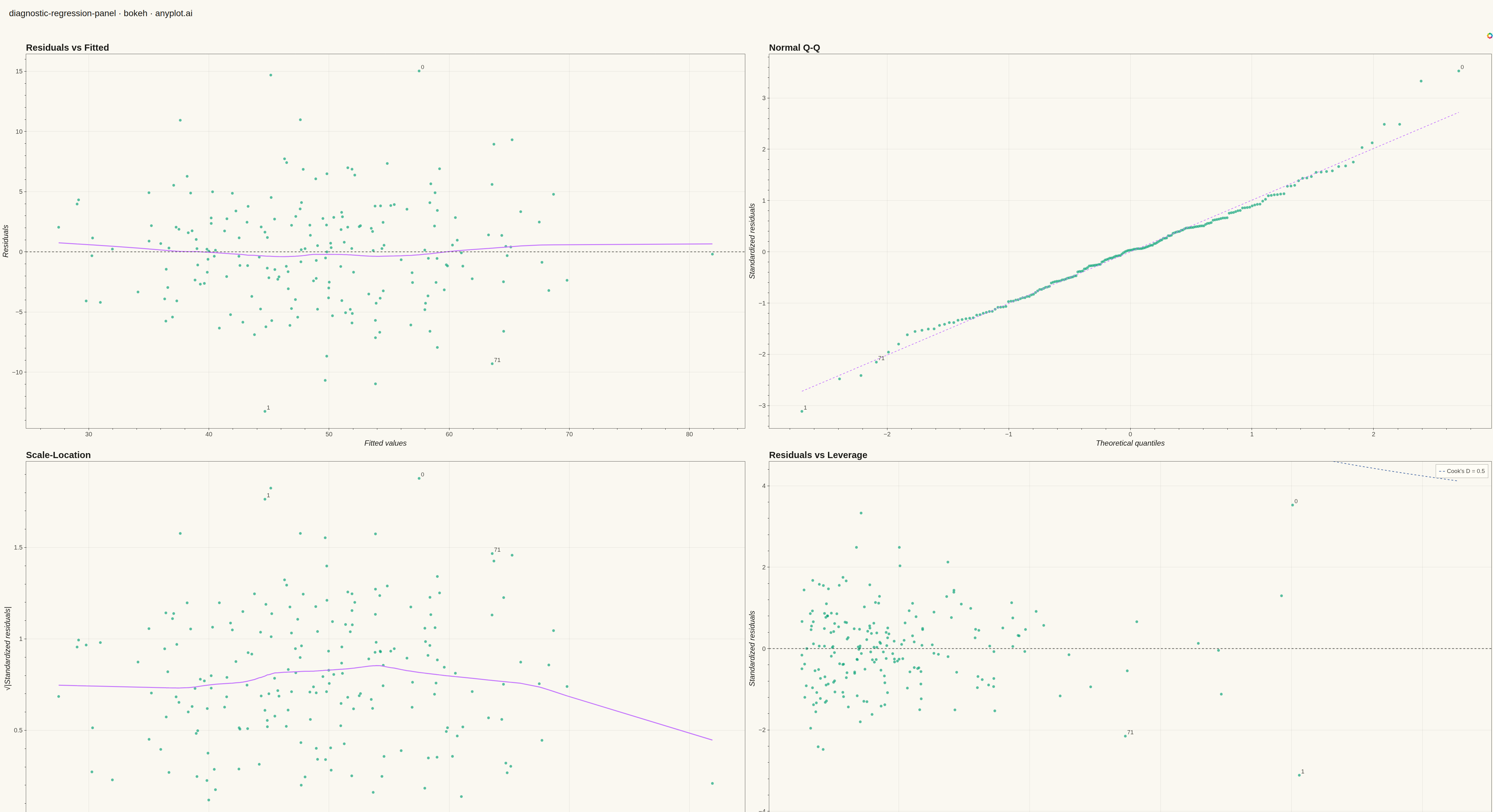
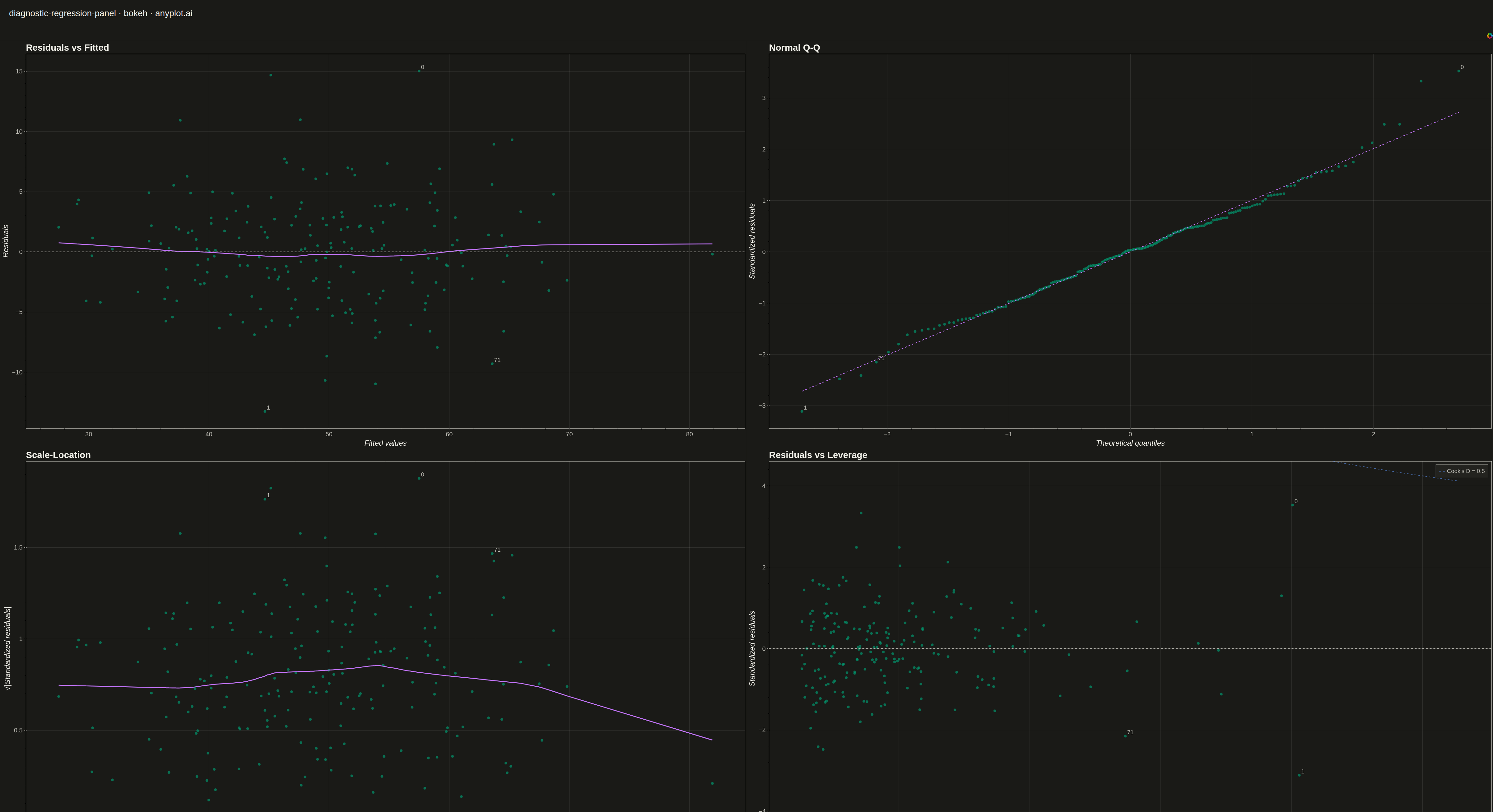
The same plot in 14 other libraries — Python: Altair, lets-plot, Matplotlib, Plotly, plotnine, Pygal, Seaborn; R: ggplot2; Julia: Makie.jl; JavaScript: Chart.js, D3.js, Apache ECharts, Highcharts, MUI X Charts. Compare all 15 side by side: Regression Diagnostic Panel (Four-Plot Display) in Python, R, Julia and JavaScript.
A 2x2 panel of diagnostic plots for evaluating linear regression model assumptions, replicating the classic output of R's `plot(lm)`. The four subplots are: (1) Residuals vs Fitted values to detect non-linearity and heteroscedasticity, (2) Normal Q-Q plot of standardized residuals to assess normality, (3) Scale-Location plot (square root of standardized residuals vs fitted values) to check homoscedasticity, and (4) Residuals vs Leverage with Cook's distance contours to identify influential observations. This composite display is the standard first step in regression model validation across statistics, academia, and regulated industries.
""" anyplot.ai
diagnostic-regression-panel: Regression Diagnostic Panel (Four-Plot Display)
Library: bokeh 3.9.0 | Python 3.13.13
Quality: 83/100 | Created: 2026-05-13
"""

import os
import sys
import time
from pathlib import Path


# Remove the script's own directory from sys.path so "bokeh" resolves to the
# installed package, not this file.
_this_dir = str(Path(__file__).parent.resolve())
sys.path = [p for p in sys.path if os.path.abspath(p) != _this_dir and p != ""]

import numpy as np
from bokeh.layouts import column, gridplot
from bokeh.models import Div, Label, Range1d, Span
from bokeh.plotting import figure, output_file, save
from scipy.stats import probplot
from selenium import webdriver
from selenium.webdriver.chrome.options import Options
from sklearn.linear_model import LinearRegression
from statsmodels.nonparametric.smoothers_lowess import lowess


# Theme tokens
THEME = os.getenv("ANYPLOT_THEME", "light")
PAGE_BG = "#FAF8F1" if THEME == "light" else "#1A1A17"
ELEVATED_BG = "#FFFDF6" if THEME == "light" else "#242420"
INK = "#1A1A17" if THEME == "light" else "#F0EFE8"
INK_SOFT = "#4A4A44" if THEME == "light" else "#B8B7B0"

BRAND = "#009E73"  # Okabe-Ito pos 1 — scatter points
ACCENT = "#C475FD"  # Okabe-Ito pos 2 — LOWESS / Q-Q reference line
BLUE = "#4467A3"  # Okabe-Ito pos 3 — Cook's distance contours

# Data: Drug-response study — standardised predictors for controlled leverage
np.random.seed(42)
n = 200
# Standardised predictors (zero mean, unit variance in the bulk)
log_dose = np.random.normal(0, 1, n)  # log-dose (standardised)
body_mass = np.random.normal(0, 1, n)  # body-mass index (standardised)
age_std = np.random.normal(0, 1, n)  # patient age (standardised)

# Two points at 2.5–3 SD from centre in predictor space → leverage ≈ 0.12–0.17
log_dose[0] = 3.0
body_mass[0] = 2.5
age_std[0] = -2.0
log_dose[1] = -2.8
body_mass[1] = -2.2
age_std[1] = 2.5

X = np.column_stack([log_dose, body_mass, age_std])
n_params = X.shape[1] + 1
X_design = np.column_stack([np.ones(n), X])

noise_sd = 4.0
response = 50 + 8 * log_dose - 5 * body_mass + 3 * age_std + np.random.normal(0, noise_sd, n)
response[0] += 14.0  # 3.5-sigma residual at high leverage → Cook's D > 0.5
response[1] -= 11.0  # 2.75-sigma residual at moderate leverage
response[70] += 10.0  # residual outlier at low leverage

# Fit linear regression
model = LinearRegression().fit(X, response)
fitted = model.predict(X)
residuals = response - fitted

# Leverage (hat matrix diagonal)
H_mat = X_design @ np.linalg.inv(X_design.T @ X_design) @ X_design.T
leverage = np.diag(H_mat)

# Standardised residuals
mse = np.sum(residuals**2) / (n - n_params)
std_residuals = residuals / np.sqrt(mse * (1 - leverage))

# Cook's distance
cooks_d = (std_residuals**2 * leverage) / (n_params * (1 - leverage))

# LOWESS smoothers for panels 1 and 3
sqrt_abs_std = np.sqrt(np.abs(std_residuals))
lowess_1 = lowess(residuals, fitted, frac=0.5, return_sorted=True)
lowess_3 = lowess(sqrt_abs_std, fitted, frac=0.5, return_sorted=True)

# Q-Q plot data
(th_q, samp_q), (qq_slope, qq_intercept, _) = probplot(std_residuals, dist="norm")

# Top 3 most influential observations by Cook's distance
top3 = np.argsort(cooks_d)[-3:][::-1]

# Map observation index → position in sorted std_residuals (for Q-Q labels)
rank_map = {int(obs): rank for rank, obs in enumerate(np.argsort(std_residuals))}

PW, PH = 2400, 1310  # per-panel pixel dimensions

# ── Panel 1: Residuals vs Fitted ──────────────────────────────────────────────
p1 = figure(
    width=PW,
    height=PH,
    title="Residuals vs Fitted",
    x_axis_label="Fitted values",
    y_axis_label="Residuals",
    background_fill_color=PAGE_BG,
    border_fill_color=PAGE_BG,
    outline_line_color=INK_SOFT,
    toolbar_location=None,
)
p1.title.text_font_size = "22pt"
p1.title.text_color = INK
p1.title.text_font_style = "bold"
p1.xaxis.axis_label_text_font_size = "18pt"
p1.yaxis.axis_label_text_font_size = "18pt"
p1.xaxis.major_label_text_font_size = "15pt"
p1.yaxis.major_label_text_font_size = "15pt"
p1.xaxis.axis_label_text_color = INK
p1.yaxis.axis_label_text_color = INK
p1.xaxis.major_label_text_color = INK_SOFT
p1.yaxis.major_label_text_color = INK_SOFT
p1.xaxis.axis_line_color = INK_SOFT
p1.yaxis.axis_line_color = INK_SOFT
p1.xaxis.major_tick_line_color = INK_SOFT
p1.yaxis.major_tick_line_color = INK_SOFT
p1.xgrid.grid_line_color = INK
p1.ygrid.grid_line_color = INK
p1.xgrid.grid_line_alpha = 0.10
p1.ygrid.grid_line_alpha = 0.10

p1.scatter(fitted, residuals, color=BRAND, size=9, alpha=0.65, line_color=PAGE_BG, line_width=0.5)
p1.add_layout(Span(location=0, dimension="width", line_color=INK_SOFT, line_dash="dashed", line_width=2))
p1.line(lowess_1[:, 0], lowess_1[:, 1], color=ACCENT, line_width=3)
for idx in top3:
    p1.add_layout(
        Label(
            x=float(fitted[idx]),
            y=float(residuals[idx]),
            text=str(int(idx)),
            text_font_size="14pt",
            text_color=INK_SOFT,
            x_offset=6,
            y_offset=6,
        )
    )

# ── Panel 2: Normal Q-Q ───────────────────────────────────────────────────────
p2 = figure(
    width=PW,
    height=PH,
    title="Normal Q-Q",
    x_axis_label="Theoretical quantiles",
    y_axis_label="Standardized residuals",
    background_fill_color=PAGE_BG,
    border_fill_color=PAGE_BG,
    outline_line_color=INK_SOFT,
    toolbar_location=None,
)
p2.title.text_font_size = "22pt"
p2.title.text_color = INK
p2.title.text_font_style = "bold"
p2.xaxis.axis_label_text_font_size = "18pt"
p2.yaxis.axis_label_text_font_size = "18pt"
p2.xaxis.major_label_text_font_size = "15pt"
p2.yaxis.major_label_text_font_size = "15pt"
p2.xaxis.axis_label_text_color = INK
p2.yaxis.axis_label_text_color = INK
p2.xaxis.major_label_text_color = INK_SOFT
p2.yaxis.major_label_text_color = INK_SOFT
p2.xaxis.axis_line_color = INK_SOFT
p2.yaxis.axis_line_color = INK_SOFT
p2.xaxis.major_tick_line_color = INK_SOFT
p2.yaxis.major_tick_line_color = INK_SOFT
p2.xgrid.grid_line_color = INK
p2.ygrid.grid_line_color = INK
p2.xgrid.grid_line_alpha = 0.10
p2.ygrid.grid_line_alpha = 0.10

p2.scatter(th_q, samp_q, color=BRAND, size=9, alpha=0.65, line_color=PAGE_BG, line_width=0.5)
qq_x_line = np.array([th_q.min(), th_q.max()])
p2.line(qq_x_line, qq_slope * qq_x_line + qq_intercept, color=ACCENT, line_width=2, line_dash="dashed")
for idx in top3:
    rank = rank_map[int(idx)]
    p2.add_layout(
        Label(
            x=float(th_q[rank]),
            y=float(samp_q[rank]),
            text=str(int(idx)),
            text_font_size="14pt",
            text_color=INK_SOFT,
            x_offset=6,
            y_offset=6,
        )
    )

# ── Panel 3: Scale-Location ───────────────────────────────────────────────────
p3 = figure(
    width=PW,
    height=PH,
    title="Scale-Location",
    x_axis_label="Fitted values",
    y_axis_label="√|Standardized residuals|",
    background_fill_color=PAGE_BG,
    border_fill_color=PAGE_BG,
    outline_line_color=INK_SOFT,
    toolbar_location=None,
)
p3.title.text_font_size = "22pt"
p3.title.text_color = INK
p3.title.text_font_style = "bold"
p3.xaxis.axis_label_text_font_size = "18pt"
p3.yaxis.axis_label_text_font_size = "18pt"
p3.xaxis.major_label_text_font_size = "15pt"
p3.yaxis.major_label_text_font_size = "15pt"
p3.xaxis.axis_label_text_color = INK
p3.yaxis.axis_label_text_color = INK
p3.xaxis.major_label_text_color = INK_SOFT
p3.yaxis.major_label_text_color = INK_SOFT
p3.xaxis.axis_line_color = INK_SOFT
p3.yaxis.axis_line_color = INK_SOFT
p3.xaxis.major_tick_line_color = INK_SOFT
p3.yaxis.major_tick_line_color = INK_SOFT
p3.xgrid.grid_line_color = INK
p3.ygrid.grid_line_color = INK
p3.xgrid.grid_line_alpha = 0.10
p3.ygrid.grid_line_alpha = 0.10

p3.scatter(fitted, sqrt_abs_std, color=BRAND, size=9, alpha=0.65, line_color=PAGE_BG, line_width=0.5)
p3.line(lowess_3[:, 0], lowess_3[:, 1], color=ACCENT, line_width=3)
for idx in top3:
    p3.add_layout(
        Label(
            x=float(fitted[idx]),
            y=float(sqrt_abs_std[idx]),
            text=str(int(idx)),
            text_font_size="14pt",
            text_color=INK_SOFT,
            x_offset=6,
            y_offset=6,
        )
    )

# ── Panel 4: Residuals vs Leverage ────────────────────────────────────────────
p4 = figure(
    width=PW,
    height=PH,
    title="Residuals vs Leverage",
    x_axis_label="Leverage",
    y_axis_label="Standardized residuals",
    background_fill_color=PAGE_BG,
    border_fill_color=PAGE_BG,
    outline_line_color=INK_SOFT,
    toolbar_location=None,
)
p4.title.text_font_size = "22pt"
p4.title.text_color = INK
p4.title.text_font_style = "bold"
p4.xaxis.axis_label_text_font_size = "18pt"
p4.yaxis.axis_label_text_font_size = "18pt"
p4.xaxis.major_label_text_font_size = "15pt"
p4.yaxis.major_label_text_font_size = "15pt"
p4.xaxis.axis_label_text_color = INK
p4.yaxis.axis_label_text_color = INK
p4.xaxis.major_label_text_color = INK_SOFT
p4.yaxis.major_label_text_color = INK_SOFT
p4.xaxis.axis_line_color = INK_SOFT
p4.yaxis.axis_line_color = INK_SOFT
p4.xaxis.major_tick_line_color = INK_SOFT
p4.yaxis.major_tick_line_color = INK_SOFT
p4.xgrid.grid_line_color = INK
p4.ygrid.grid_line_color = INK
p4.xgrid.grid_line_alpha = 0.10
p4.ygrid.grid_line_alpha = 0.10

# Constrain y-axis so Cook's D contours are visible even when outliers are extreme
p4_ylim = max(4.0, float(np.percentile(np.abs(std_residuals), 96))) * 1.15
p4.y_range = Range1d(-p4_ylim, p4_ylim)

p4.scatter(leverage, std_residuals, color=BRAND, size=9, alpha=0.65, line_color=PAGE_BG, line_width=0.5)
p4.add_layout(Span(location=0, dimension="width", line_color=INK_SOFT, line_dash="dashed", line_width=2))

lev_range = np.linspace(1e-4, min(float(leverage.max()) * 1.3, 0.99), 400)
for cook_level, dash, leg_lbl in [(0.5, "dashed", "Cook's D = 0.5"), (1.0, "dotted", "Cook's D = 1.0")]:
    cook_y = np.sqrt(np.abs(cook_level * n_params * (1 - lev_range) / lev_range))
    # Clip to visible range to avoid rendering artifacts
    visible = cook_y <= p4_ylim * 1.05
    if np.any(visible):
        p4.line(lev_range[visible], cook_y[visible], color=BLUE, line_width=2, line_dash=dash, legend_label=leg_lbl)
        p4.line(lev_range[visible], -cook_y[visible], color=BLUE, line_width=2, line_dash=dash)

for idx in top3:
    sr = float(std_residuals[idx])
    # Only label if within the visible y-range
    if abs(sr) <= p4_ylim:
        p4.add_layout(
            Label(
                x=float(leverage[idx]),
                y=sr,
                text=str(int(idx)),
                text_font_size="14pt",
                text_color=INK_SOFT,
                x_offset=6,
                y_offset=6,
            )
        )

p4.legend.background_fill_color = ELEVATED_BG
p4.legend.border_line_color = INK_SOFT
p4.legend.label_text_color = INK_SOFT
p4.legend.label_text_font_size = "14pt"

# ── Assemble and export ───────────────────────────────────────────────────────
grid = gridplot([[p1, p2], [p3, p4]], merge_tools=False)

title_div = Div(
    text=(
        f'<div style="font-family: sans-serif; font-size: 28px; font-weight: 500;'
        f' color: {INK}; background-color: {PAGE_BG}; padding: 18px 24px 6px 24px; margin: 0;">'
        f"diagnostic-regression-panel · bokeh · anyplot.ai</div>"
    ),
    width=4800,
    height=90,
)

layout = column(title_div, grid)
output_file(f"plot-{THEME}.html")
save(layout)

W_SCR, H_SCR = 4800, 2750
opts = Options()
for arg in (
    "--headless=new",
    "--no-sandbox",
    "--disable-dev-shm-usage",
    "--disable-gpu",
    f"--window-size={W_SCR},{H_SCR}",
    "--hide-scrollbars",
):
    opts.add_argument(arg)
driver = webdriver.Chrome(options=opts)
driver.set_window_size(W_SCR, H_SCR)
driver.get(f"file://{Path(f'plot-{THEME}.html').resolve()}")
time.sleep(3)
driver.execute_script(
    f"document.body.style.backgroundColor='{PAGE_BG}';"
    f"document.body.style.margin='0';"
    f"document.documentElement.style.backgroundColor='{PAGE_BG}';"
)
driver.save_screenshot(f"plot-{THEME}.png")
driver.quit()
Runnable source as JSON, for any HTTP client: https://api.anyplot.ai/specs/diagnostic-regression-panel/bokeh/code. Any spec id and library id listed in llms-full.txt fit the same URL shape; every URL below is complete and callable.
{
  "spec_id": "diagnostic-regression-panel",
  "language": "python",
  "library": "bokeh",
  "page": "https://anyplot.ai/diagnostic-regression-panel/python/bokeh",
  "hub": "https://anyplot.ai/diagnostic-regression-panel",
  "code_json": "https://api.anyplot.ai/specs/diagnostic-regression-panel/bokeh/code",
  "spec_json": "https://api.anyplot.ai/specs/diagnostic-regression-panel",
  "render_light_png": "https://storage.googleapis.com/anyplot-images/plots/diagnostic-regression-panel/python/bokeh/plot-light.png",
  "render_dark_png": "https://storage.googleapis.com/anyplot-images/plots/diagnostic-regression-panel/python/bokeh/plot-dark.png",
  "interactive_light_html": "https://storage.googleapis.com/anyplot-images/plots/diagnostic-regression-panel/python/bokeh/plot-light.html",
  "interactive_dark_html": "https://storage.googleapis.com/anyplot-images/plots/diagnostic-regression-panel/python/bokeh/plot-dark.html",
  "quality_score": 83.0,
  "license": "MIT",
  "guide": "https://anyplot.ai/llms.txt"
}
Part of Regression Diagnostic Panel (Four-Plot Display) on anyplot.ai.