The same plot in 14 other libraries — JavaScript: Chart.js, D3.js, Highcharts, MUI X Charts; Python: Altair, Bokeh, lets-plot, Matplotlib, Plotly, plotnine, Pygal, Seaborn; R: ggplot2; Julia: Makie.jl. Compare all 15 side by side: Regression Diagnostic Panel (Four-Plot Display) in Python, R, Julia and JavaScript.
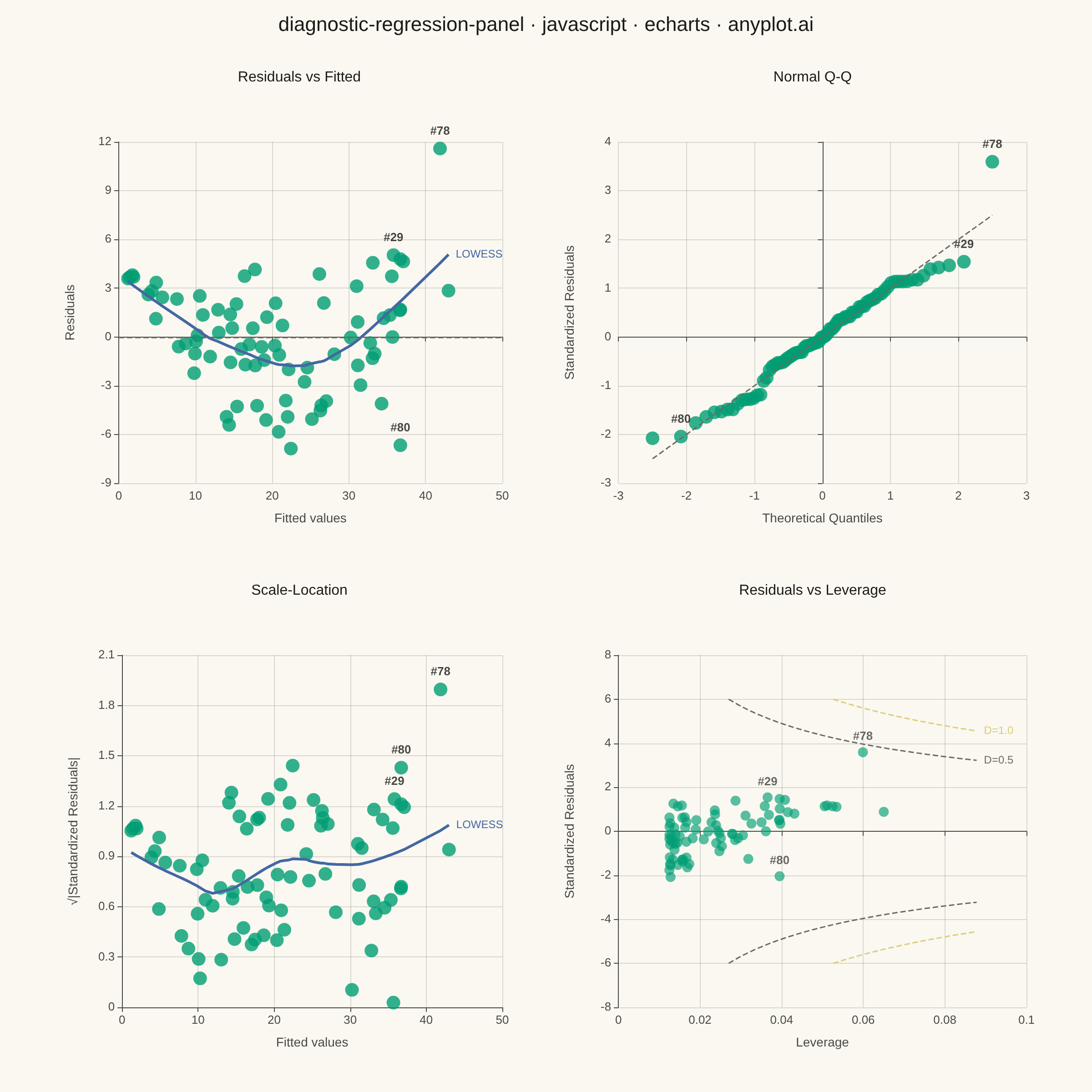
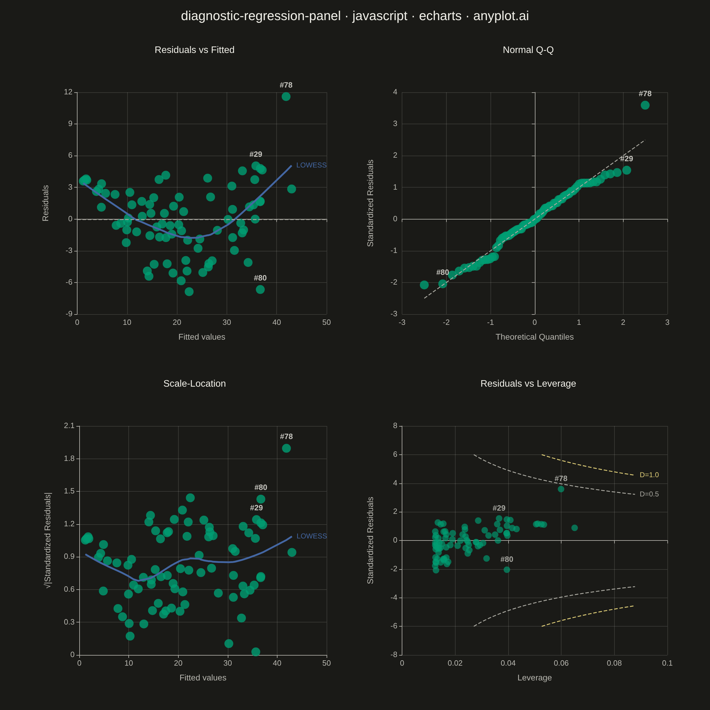
A 2x2 panel of diagnostic plots for evaluating linear regression model assumptions, replicating the classic output of R's `plot(lm)`. The four subplots are: (1) Residuals vs Fitted values to detect non-linearity and heteroscedasticity, (2) Normal Q-Q plot of standardized residuals to assess normality, (3) Scale-Location plot (square root of standardized residuals vs fitted values) to check homoscedasticity, and (4) Residuals vs Leverage with Cook's distance contours to identify influential observations. This composite display is the standard first step in regression model validation across statistics, academia, and regulated industries.
// anyplot.ai
// diagnostic-regression-panel: Regression Diagnostic Panel (Four-Plot Display)
// Library: echarts 6.1.0 | JavaScript 22.23.2
// Quality: 90/100 | Created: 2026-09-05

//# anyplot-orientation: square
const t = window.ANYPLOT_TOKENS;
// The harness doesn't expose a "muted" token — derive it locally (see
// default-style-guide.md "Theme-adaptive Chrome" semantic anchors table).
const inkMuted = t.theme === "light" ? "#6B6A63" : "#A8A79F";

// --- Deterministic PRNG (LCG + Box-Muller) ---------------------------------
function makeLcg(seed) {
  let state = seed >>> 0;
  return function uniform() {
    state = (1664525 * state + 1013904223) >>> 0;
    return state / 4294967296;
  };
}
function makeGaussian(uniform) {
  let spare = null;
  return function gaussian(mean, sd) {
    if (spare !== null) {
      const z = spare;
      spare = null;
      return mean + sd * z;
    }
    let u1 = 0;
    do {
      u1 = uniform();
    } while (u1 <= 1e-12);
    const u2 = uniform();
    const mag = Math.sqrt(-2 * Math.log(u1));
    spare = mag * Math.sin(2 * Math.PI * u2);
    return mean + sd * mag * Math.cos(2 * Math.PI * u2);
  };
}

// --- Inverse normal CDF (Acklam's rational approximation) ------------------
function qnorm(p) {
  const a = [
    -3.969683028665376e1, 2.209460984245205e2, -2.759285104469687e2,
    1.38357751867269e2, -3.066479806614716e1, 2.506628277459239,
  ];
  const b = [
    -5.447609879822406e1, 1.615858368580409e2, -1.556989798598866e2,
    6.680131188771972e1, -1.328068155288572e1,
  ];
  const c = [
    -7.784894002430293e-3, -3.223964580411365e-1, -2.400758277161838,
    -2.549732539343734, 4.374664141464968, 2.938163982698783,
  ];
  const d = [
    7.784695709041462e-3, 3.224671290700398e-1, 2.445134137142996,
    3.754408661907416,
  ];
  const plow = 0.02425;
  const phigh = 1 - plow;
  if (p < plow) {
    const q = Math.sqrt(-2 * Math.log(p));
    return (
      (((((c[0] * q + c[1]) * q + c[2]) * q + c[3]) * q + c[4]) * q + c[5]) /
      ((((d[0] * q + d[1]) * q + d[2]) * q + d[3]) * q + 1)
    );
  }
  if (p <= phigh) {
    const q = p - 0.5;
    const r = q * q;
    return (
      ((((((a[0] * r + a[1]) * r + a[2]) * r + a[3]) * r + a[4]) * r + a[5]) *
        q) /
      (((((b[0] * r + b[1]) * r + b[2]) * r + b[3]) * r + b[4]) * r + 1)
    );
  }
  const q = Math.sqrt(-2 * Math.log(1 - p));
  return (
    -(((((c[0] * q + c[1]) * q + c[2]) * q + c[3]) * q + c[4]) * q + c[5]) /
    ((((d[0] * q + d[1]) * q + d[2]) * q + d[3]) * q + 1)
  );
}

// --- Local-linear LOWESS smoother -------------------------------------------
function lowess(xValues, yValues, frac) {
  const n = xValues.length;
  const window = Math.max(3, Math.floor(frac * n));
  const order = xValues
    .map((_, i) => i)
    .sort((a, b) => xValues[a] - xValues[b]);
  const sortedX = order.map((i) => xValues[i]);
  const sortedY = order.map((i) => yValues[i]);
  const fitted = new Array(n);
  for (let i = 0; i < n; i += 1) {
    const x0 = sortedX[i];
    const distances = sortedX.map((x) => Math.abs(x - x0));
    const bandwidth = [...distances].sort((a, b) => a - b)[window - 1] || 1;
    let sumW = 0;
    let sumWx = 0;
    let sumWy = 0;
    let sumWxy = 0;
    let sumWxx = 0;
    for (let j = 0; j < n; j += 1) {
      const ratio = Math.min(1, distances[j] / bandwidth);
      const w = (1 - ratio ** 3) ** 3;
      sumW += w;
      sumWx += w * sortedX[j];
      sumWy += w * sortedY[j];
      sumWxy += w * sortedX[j] * sortedY[j];
      sumWxx += w * sortedX[j] * sortedX[j];
    }
    const denom = sumW * sumWxx - sumWx * sumWx;
    const slope =
      Math.abs(denom) < 1e-9 ? 0 : (sumW * sumWxy - sumWx * sumWy) / denom;
    const intercept = (sumWy - slope * sumWx) / sumW;
    fitted[i] = intercept + slope * x0;
  }
  return sortedX.map((x, i) => [x, fitted[i]]);
}

// --- Data: simulate a regression with heteroscedasticity, mild curvature ---
// and two crafted high-leverage points (one influential, one not) ----------
const uniform = makeLcg(42);
const gaussian = makeGaussian(uniform);

const predictor = [];
const response = [];
for (let i = 0; i < 77; i += 1) {
  const x = uniform() * 10;
  const noiseSd = 0.6 + 0.35 * x;
  const trueY = 5 + 1.8 * x + 0.15 * x * x;
  predictor.push(x);
  response.push(trueY + gaussian(0, noiseSd));
}
predictor.push(11.2);
response.push(5 + 1.8 * 11.2 + 0.15 * 11.2 * 11.2 + 9.5); // high leverage + large residual -> influential
predictor.push(11.5);
response.push(5 + 1.8 * 11.5 + 0.15 * 11.5 * 11.5 + 0.3); // high leverage, small residual -> not influential
predictor.push(9.8);
response.push(5 + 1.8 * 9.8 + 0.15 * 9.8 * 9.8 - 7.0); // moderate leverage, large negative residual
const n = predictor.length;

// --- Simple linear regression (least squares) -------------------------------
const meanX = predictor.reduce((a, v) => a + v, 0) / n;
const meanY = response.reduce((a, v) => a + v, 0) / n;
let sumSquaredX = 0;
let sumCrossXY = 0;
for (let i = 0; i < n; i += 1) {
  const dx = predictor[i] - meanX;
  sumSquaredX += dx * dx;
  sumCrossXY += dx * (response[i] - meanY);
}
const slope = sumCrossXY / sumSquaredX;
const intercept = meanY - slope * meanX;

const fittedValues = predictor.map((x) => intercept + slope * x);
const residuals = response.map((y, i) => y - fittedValues[i]);

const numParams = 2; // intercept + slope
let sumSquaredResid = 0;
residuals.forEach((r) => {
  sumSquaredResid += r * r;
});
const residualScale = Math.sqrt(sumSquaredResid / (n - numParams));

const leverage = predictor.map((x) => 1 / n + (x - meanX) ** 2 / sumSquaredX);
const standardizedResiduals = residuals.map(
  (r, i) => r / (residualScale * Math.sqrt(1 - leverage[i])),
);
const sqrtAbsStdResiduals = standardizedResiduals.map((r) =>
  Math.sqrt(Math.abs(r)),
);
const cooksDistance = standardizedResiduals.map(
  (r, i) => (r * r * leverage[i]) / (numParams * (1 - leverage[i])),
);

const rankByCooksD = predictor
  .map((_, i) => i)
  .sort((a, b) => cooksDistance[b] - cooksDistance[a]);
const influentialIdx = new Set(rankByCooksD.slice(0, 3));

function withInfluentialLabel(x, y, obsIdx) {
  if (!influentialIdx.has(obsIdx)) return [x, y];
  return {
    value: [x, y],
    label: {
      show: true,
      formatter: `#${obsIdx + 1}`,
      position: "top",
      color: t.ink,
      fontSize: 13,
      fontWeight: "bold",
    },
  };
}

// --- Subplot 1: Residuals vs Fitted -----------------------------------------
const residualsVsFittedData = predictor.map((x, i) =>
  withInfluentialLabel(fittedValues[i], residuals[i], i),
);
const residualsLowess = lowess(fittedValues, residuals, 0.6);

// --- Subplot 2: Normal Q-Q ---------------------------------------------------
const sortedByStdResid = standardizedResiduals
  .map((_, i) => i)
  .sort((a, b) => standardizedResiduals[a] - standardizedResiduals[b]);
const qqData = sortedByStdResid.map((obsIdx, rank) => {
  const theoreticalQuantile = qnorm((rank + 0.5) / n);
  return withInfluentialLabel(
    theoreticalQuantile,
    standardizedResiduals[obsIdx],
    obsIdx,
  );
});
const theoreticalQuantiles = sortedByStdResid.map((_, rank) =>
  qnorm((rank + 0.5) / n),
);
const qqRange = [
  Math.min(...theoreticalQuantiles),
  Math.max(...theoreticalQuantiles),
];

// --- Subplot 3: Scale-Location -----------------------------------------------
const scaleLocationData = predictor.map((x, i) =>
  withInfluentialLabel(fittedValues[i], sqrtAbsStdResiduals[i], i),
);
const scaleLocationLowess = lowess(fittedValues, sqrtAbsStdResiduals, 0.6);

// --- Subplot 4: Residuals vs Leverage, with Cook's distance contours --------
const residualsVsLeverageData = predictor.map((x, i) =>
  withInfluentialLabel(leverage[i], standardizedResiduals[i], i),
);
const maxLeverage = Math.max(...leverage);
const maxAbsStdResid = Math.max(...standardizedResiduals.map(Math.abs));
const contourHMax = Math.min(0.85, maxLeverage * 1.35);
const contourYCap = Math.max(6, maxAbsStdResid + 1);

function cooksContourBranch(cooksD, sign) {
  const hMin =
    (cooksD * numParams) / (contourYCap * contourYCap + cooksD * numParams);
  const points = [];
  const steps = 50;
  for (let i = 0; i <= steps; i += 1) {
    const h = hMin + (contourHMax - hMin) * (i / steps);
    if (h <= 0 || h >= 1) continue;
    const underRoot = (cooksD * numParams * (1 - h)) / h;
    if (underRoot < 0) continue;
    points.push([h, sign * Math.sqrt(underRoot)]);
  }
  return points;
}

// --- Layout: 2x2 grid of subplots, shared figure title ----------------------
const gridBoxes = [
  { left: "9%", right: "54%", top: "13%", bottom: "54%" },
  { left: "55%", right: "6%", top: "13%", bottom: "54%" },
  { left: "9%", right: "54%", top: "60%", bottom: "6%" },
  { left: "55%", right: "6%", top: "60%", bottom: "6%" },
];
const subplotTitles = [
  { text: "Residuals vs Fitted", left: "27%", top: "6%" },
  { text: "Normal Q-Q", left: "74%", top: "6%" },
  { text: "Scale-Location", left: "27%", top: "53%" },
  { text: "Residuals vs Leverage", left: "74%", top: "53%" },
];

const chart = echarts.init(document.getElementById("container"));
chart.setOption({
  animation: false,
  backgroundColor: "transparent",
  title: [
    {
      text: "diagnostic-regression-panel · javascript · echarts · anyplot.ai",
      left: "center",
      top: "1%",
      textStyle: { color: t.ink, fontSize: 22, fontWeight: 500 },
    },
    ...subplotTitles.map((cfg) => ({
      text: cfg.text,
      left: cfg.left,
      top: cfg.top,
      textAlign: "center",
      textStyle: { color: t.ink, fontSize: 16, fontWeight: 500 },
    })),
  ],
  grid: gridBoxes.map((box) => ({ ...box, containLabel: true })),
  xAxis: [
    {
      gridIndex: 0,
      type: "value",
      name: "Fitted values",
      nameLocation: "middle",
      nameGap: 32,
      nameTextStyle: { color: t.inkSoft, fontSize: 14 },
      axisLabel: { color: t.inkSoft, fontSize: 13 },
      axisLine: { lineStyle: { color: t.inkSoft } },
      splitLine: { lineStyle: { color: t.grid } },
    },
    {
      gridIndex: 1,
      type: "value",
      name: "Theoretical Quantiles",
      nameLocation: "middle",
      nameGap: 32,
      nameTextStyle: { color: t.inkSoft, fontSize: 14 },
      axisLabel: { color: t.inkSoft, fontSize: 13 },
      axisLine: { lineStyle: { color: t.inkSoft } },
      splitLine: { lineStyle: { color: t.grid } },
    },
    {
      gridIndex: 2,
      type: "value",
      name: "Fitted values",
      nameLocation: "middle",
      nameGap: 32,
      nameTextStyle: { color: t.inkSoft, fontSize: 14 },
      axisLabel: { color: t.inkSoft, fontSize: 13 },
      axisLine: { lineStyle: { color: t.inkSoft } },
      splitLine: { lineStyle: { color: t.grid } },
    },
    {
      gridIndex: 3,
      type: "value",
      name: "Leverage",
      nameLocation: "middle",
      nameGap: 32,
      min: 0,
      nameTextStyle: { color: t.inkSoft, fontSize: 14 },
      axisLabel: { color: t.inkSoft, fontSize: 13 },
      axisLine: { lineStyle: { color: t.inkSoft } },
      splitLine: { lineStyle: { color: t.grid } },
    },
  ],
  yAxis: [
    {
      gridIndex: 0,
      type: "value",
      name: "Residuals",
      nameLocation: "middle",
      nameGap: 46,
      nameTextStyle: { color: t.inkSoft, fontSize: 14 },
      axisLabel: { color: t.inkSoft, fontSize: 13 },
      axisLine: { lineStyle: { color: t.inkSoft } },
      splitLine: { lineStyle: { color: t.grid } },
    },
    {
      gridIndex: 1,
      type: "value",
      name: "Standardized Residuals",
      nameLocation: "middle",
      nameGap: 46,
      nameTextStyle: { color: t.inkSoft, fontSize: 14 },
      axisLabel: { color: t.inkSoft, fontSize: 13 },
      axisLine: { lineStyle: { color: t.inkSoft } },
      splitLine: { lineStyle: { color: t.grid } },
    },
    {
      gridIndex: 2,
      type: "value",
      name: "√|Standardized Residuals|",
      nameLocation: "middle",
      nameGap: 46,
      nameTextStyle: { color: t.inkSoft, fontSize: 14 },
      axisLabel: { color: t.inkSoft, fontSize: 13 },
      axisLine: { lineStyle: { color: t.inkSoft } },
      splitLine: { lineStyle: { color: t.grid } },
    },
    {
      gridIndex: 3,
      type: "value",
      name: "Standardized Residuals",
      nameLocation: "middle",
      nameGap: 46,
      nameTextStyle: { color: t.inkSoft, fontSize: 14 },
      axisLabel: { color: t.inkSoft, fontSize: 13 },
      axisLine: { lineStyle: { color: t.inkSoft } },
      splitLine: { lineStyle: { color: t.grid } },
    },
  ],
  series: [
    // Subplot 1: Residuals vs Fitted
    {
      type: "scatter",
      xAxisIndex: 0,
      yAxisIndex: 0,
      data: residualsVsFittedData,
      symbolSize: 15,
      itemStyle: { color: t.palette[0], opacity: 0.8 },
      markLine: {
        silent: true,
        symbol: "none",
        label: { show: false },
        lineStyle: { color: inkMuted, type: "dashed", width: 1.5 },
        data: [{ yAxis: 0 }],
      },
    },
    {
      type: "line",
      xAxisIndex: 0,
      yAxisIndex: 0,
      data: residualsLowess,
      showSymbol: false,
      silent: true,
      lineStyle: { color: t.palette[2], width: 3 },
      endLabel: {
        show: true,
        formatter: "LOWESS",
        color: t.palette[2],
        fontSize: 12,
      },
    },
    // Subplot 2: Normal Q-Q
    {
      type: "scatter",
      xAxisIndex: 1,
      yAxisIndex: 1,
      data: qqData,
      symbolSize: 15,
      itemStyle: { color: t.palette[0], opacity: 0.8 },
      markLine: {
        silent: true,
        symbol: "none",
        label: { show: false },
        lineStyle: { color: inkMuted, type: "dashed", width: 1.5 },
        data: [
          [
            { coord: [qqRange[0], qqRange[0]] },
            { coord: [qqRange[1], qqRange[1]] },
          ],
        ],
      },
    },
    // Subplot 3: Scale-Location
    {
      type: "scatter",
      xAxisIndex: 2,
      yAxisIndex: 2,
      data: scaleLocationData,
      symbolSize: 15,
      itemStyle: { color: t.palette[0], opacity: 0.8 },
    },
    {
      type: "line",
      xAxisIndex: 2,
      yAxisIndex: 2,
      data: scaleLocationLowess,
      showSymbol: false,
      silent: true,
      lineStyle: { color: t.palette[2], width: 3 },
      endLabel: {
        show: true,
        formatter: "LOWESS",
        color: t.palette[2],
        fontSize: 12,
      },
    },
    // Subplot 4: Residuals vs Leverage, with Cook's distance contours
    {
      type: "scatter",
      xAxisIndex: 3,
      yAxisIndex: 3,
      data: residualsVsLeverageData,
      symbolSize: 11,
      itemStyle: { color: t.palette[0], opacity: 0.65 },
    },
    {
      type: "line",
      xAxisIndex: 3,
      yAxisIndex: 3,
      data: cooksContourBranch(0.5, 1),
      showSymbol: false,
      silent: true,
      lineStyle: { color: inkMuted, type: "dashed", width: 1.5 },
      endLabel: {
        show: true,
        formatter: "D=0.5",
        color: inkMuted,
        fontSize: 12,
      },
    },
    {
      type: "line",
      xAxisIndex: 3,
      yAxisIndex: 3,
      data: cooksContourBranch(0.5, -1),
      showSymbol: false,
      silent: true,
      lineStyle: { color: inkMuted, type: "dashed", width: 1.5 },
    },
    {
      type: "line",
      xAxisIndex: 3,
      yAxisIndex: 3,
      data: cooksContourBranch(1.0, 1),
      showSymbol: false,
      silent: true,
      lineStyle: { color: t.amber, type: "dashed", width: 1.5 },
      endLabel: {
        show: true,
        formatter: "D=1.0",
        color: t.amber,
        fontSize: 12,
      },
    },
    {
      type: "line",
      xAxisIndex: 3,
      yAxisIndex: 3,
      data: cooksContourBranch(1.0, -1),
      showSymbol: false,
      silent: true,
      lineStyle: { color: t.amber, type: "dashed", width: 1.5 },
    },
  ],
});
Runnable source as JSON, for any HTTP client: https://api.anyplot.ai/specs/diagnostic-regression-panel/echarts/code. Any spec id and library id listed in llms-full.txt fit the same URL shape; every URL below is complete and callable.
{
  "spec_id": "diagnostic-regression-panel",
  "language": "javascript",
  "library": "echarts",
  "page": "https://anyplot.ai/diagnostic-regression-panel/javascript/echarts",
  "hub": "https://anyplot.ai/diagnostic-regression-panel",
  "code_json": "https://api.anyplot.ai/specs/diagnostic-regression-panel/echarts/code",
  "spec_json": "https://api.anyplot.ai/specs/diagnostic-regression-panel",
  "render_light_png": "https://storage.googleapis.com/anyplot-images/plots/diagnostic-regression-panel/javascript/echarts/plot-light.png",
  "render_dark_png": "https://storage.googleapis.com/anyplot-images/plots/diagnostic-regression-panel/javascript/echarts/plot-dark.png",
  "interactive_light_html": "https://storage.googleapis.com/anyplot-images/plots/diagnostic-regression-panel/javascript/echarts/plot-light.html",
  "interactive_dark_html": "https://storage.googleapis.com/anyplot-images/plots/diagnostic-regression-panel/javascript/echarts/plot-dark.html",
  "quality_score": 90.0,
  "license": "MIT",
  "guide": "https://anyplot.ai/llms.txt"
}
Part of Regression Diagnostic Panel (Four-Plot Display) on anyplot.ai.