The same plot in 14 other libraries — Python: Altair, Bokeh, lets-plot, Matplotlib, Plotly, plotnine, Pygal, Seaborn; R: ggplot2; JavaScript: Chart.js, D3.js, Apache ECharts, Highcharts, MUI X Charts. Compare all 15 side by side: Regression Diagnostic Panel (Four-Plot Display) in Python, R, Julia and JavaScript.
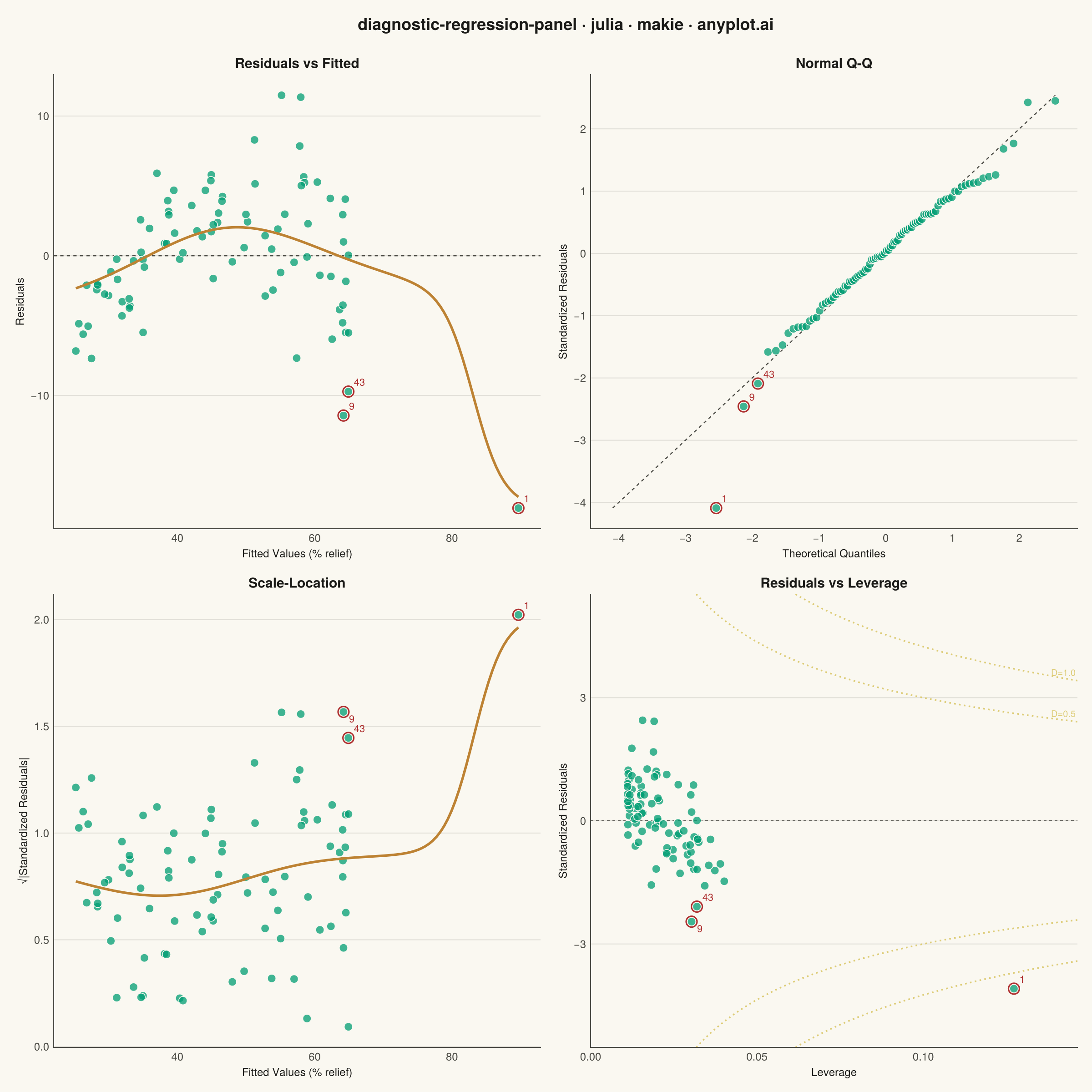
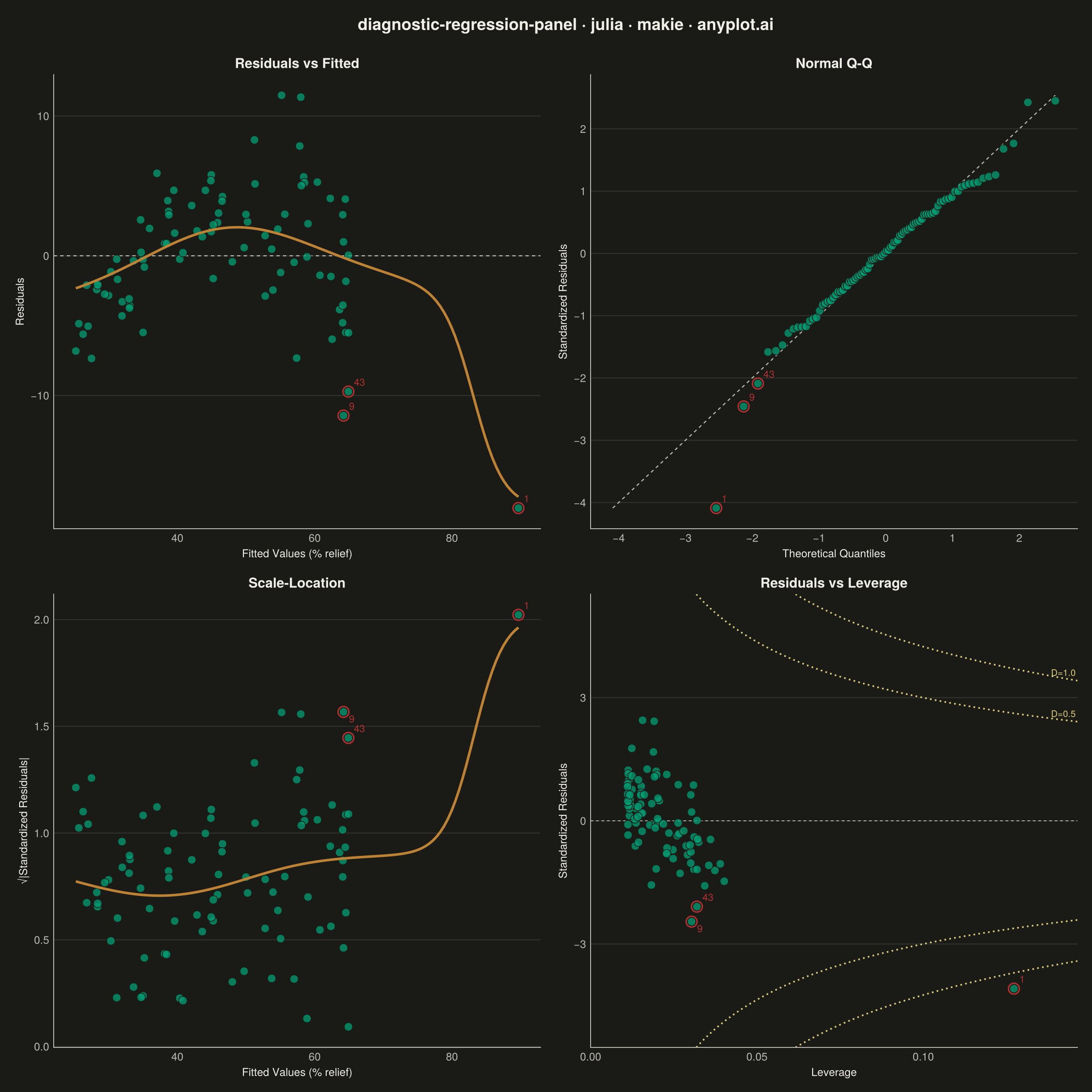
A 2x2 panel of diagnostic plots for evaluating linear regression model assumptions, replicating the classic output of R's `plot(lm)`. The four subplots are: (1) Residuals vs Fitted values to detect non-linearity and heteroscedasticity, (2) Normal Q-Q plot of standardized residuals to assess normality, (3) Scale-Location plot (square root of standardized residuals vs fitted values) to check homoscedasticity, and (4) Residuals vs Leverage with Cook's distance contours to identify influential observations. This composite display is the standard first step in regression model validation across statistics, academia, and regulated industries.
# anyplot.ai
# diagnostic-regression-panel: Regression Diagnostic Panel (Four-Plot Display)
# Library: makie 0.21.9 | Julia 1.11.9
# Quality: 88/100 | Created: 2026-09-05

using CairoMakie
using Colors
using Random
using LinearAlgebra

Random.seed!(42)

# --- Theme tokens ------------------------------------------------------------
const THEME       = get(ENV, "ANYPLOT_THEME", "light")
const PAGE_BG     = THEME == "light" ? colorant"#FAF8F1" : colorant"#1A1A17"
const ELEVATED_BG = THEME == "light" ? colorant"#FFFDF6" : colorant"#242420"
const INK         = THEME == "light" ? colorant"#1A1A17" : colorant"#F0EFE8"
const INK_SOFT    = THEME == "light" ? colorant"#4A4A44" : colorant"#B8B7B0"
const BRAND       = colorant"#009E73"  # Imprint position 1 — data points
const OCHRE       = colorant"#BD8233"  # Imprint position 4 — smoother trend
const MATTE_RED   = colorant"#AE3030"  # semantic anchor — flagged influential points
const AMBER       = colorant"#DDCC77"  # semantic anchor — Cook's distance warning contours

# --- Standard normal quantile (inverse CDF), Acklam's rational approximation --
function norm_quantile(p)
    a = (-3.969683028665376e+01, 2.209460984245205e+02, -2.759285104469687e+02,
        1.383577518672690e+02, -3.066479806614716e+01, 2.506628277459239e+00)
    b = (-5.447609879822406e+01, 1.615858368580409e+02, -1.556989798598866e+02,
        6.680131188771972e+01, -1.328068155288572e+01)
    c = (-7.784894002430293e-03, -3.223964580411365e-01, -2.400758277161838e+00,
        -2.549732539343734e+00, 4.374664141464968e+00, 2.938163982698783e+00)
    d = (7.784695709041462e-03, 3.224671290700398e-01, 2.445134137142996e+00,
        3.754408661907416e+00)
    p_low = 0.02425
    p_high = 1 - p_low
    if p < p_low
        q = sqrt(-2 * log(p))
        return (((((c[1] * q + c[2]) * q + c[3]) * q + c[4]) * q + c[5]) * q + c[6]) /
               ((((d[1] * q + d[2]) * q + d[3]) * q + d[4]) * q + 1)
    elseif p <= p_high
        q = p - 0.5
        r = q * q
        return (((((a[1] * r + a[2]) * r + a[3]) * r + a[4]) * r + a[5]) * r + a[6]) * q /
               (((((b[1] * r + b[2]) * r + b[3]) * r + b[4]) * r + b[5]) * r + 1)
    else
        q = sqrt(-2 * log(1 - p))
        return -(((((c[1] * q + c[2]) * q + c[3]) * q + c[4]) * q + c[5]) * q + c[6]) /
               ((((d[1] * q + d[2]) * q + d[3]) * q + d[4]) * q + 1)
    end
end

# --- Gaussian-kernel local regression (LOWESS-style smoother, no package) ----
function lowess_smooth(x, y, x_eval, bandwidth)
    y_smooth = similar(x_eval)
    for i in eachindex(x_eval)
        w = exp.(-((x .- x_eval[i]) ./ bandwidth) .^ 2)
        wsum = sum(w)
        y_smooth[i] = wsum > 1e-10 ? sum(w .* y) / wsum : NaN
    end
    return y_smooth
end

# --- Data: a dose-response regression with mild non-linearity, --------------
# heteroscedastic noise, and a couple of injected influential observations ---
n = 90
dose_mg = rand(n) .* 90.0 .+ 5.0                 # drug dose administered, 5-95 mg
dose_mg[1] = 150.0                               # extrapolated high-dose (high-leverage) point
dose_mg[2] = 92.0

mu = 14.0 .+ 0.85 .* dose_mg .- 0.0035 .* dose_mg .^ 2  # true response plateaus at high dose
noise_scale = 0.9 .+ 0.045 .* dose_mg             # variance grows with dose (heteroscedastic)
response_pct = mu .+ noise_scale .* randn(n)      # percent symptom relief
response_pct[1] += 10.0                           # push the high-leverage point off-trend
response_pct[3] -= 8.5                            # a second, non-leverage but large residual

# Ordinary least squares fit: response_pct ~ 1 + dose_mg
X = hcat(ones(n), dose_mg)
p = size(X, 2)
beta = X \ response_pct
fitted = X * beta
residuals = response_pct .- fitted

hat_matrix = X * inv(X' * X) * X'
leverage = diag(hat_matrix)

mse = sum(residuals .^ 2) / (n - p)
sigma_hat = sqrt(mse)
std_residuals = residuals ./ (sigma_hat .* sqrt.(1 .- leverage))
sqrt_abs_std_resid = sqrt.(abs.(std_residuals))
cooks_d = (std_residuals .^ 2 .* leverage) ./ (p .* (1 .- leverage))

ord = sortperm(std_residuals)
sorted_std_resid = std_residuals[ord]
ranks = invperm(ord)
plot_pos = ((1:n) .- 0.5) ./ n
theoretical_q = norm_quantile.(plot_pos)

top_idx = sortperm(cooks_d, rev = true)[1:3]      # 3 most influential observations

fitted_eval = collect(range(minimum(fitted), maximum(fitted), length = 120))
bw = (maximum(fitted) - minimum(fitted)) / 6
resid_smooth = lowess_smooth(fitted, residuals, fitted_eval, bw)
scale_smooth = lowess_smooth(fitted, sqrt_abs_std_resid, fitted_eval, bw)

# --- Figure -------------------------------------------------------------------
title_str = "diagnostic-regression-panel · julia · makie · anyplot.ai"

fig = Figure(size = (1200, 1200), fontsize = 14, backgroundcolor = PAGE_BG)

Label(fig[0, 1:2], title_str; fontsize = 18, color = INK, font = :bold, padding = (0, 0, 6, 0))

# --- Panel 1: Residuals vs Fitted --------------------------------------------
ax1 = Axis(
    fig[1, 1];
    title              = "Residuals vs Fitted",
    titlesize          = 15,
    titlecolor         = INK,
    xlabel             = "Fitted Values (% relief)",
    ylabel             = "Residuals",
    xlabelsize         = 12,
    ylabelsize         = 12,
    xlabelcolor        = INK,
    ylabelcolor        = INK,
    xticklabelsize     = 12,
    yticklabelsize     = 12,
    xticklabelcolor    = INK_SOFT,
    yticklabelcolor    = INK_SOFT,
    xtickcolor         = INK_SOFT,
    ytickcolor         = INK_SOFT,
    xticksize          = 0,
    yticksize          = 0,
    backgroundcolor    = PAGE_BG,
    topspinevisible    = false,
    rightspinevisible  = false,
    leftspinecolor     = INK_SOFT,
    bottomspinecolor   = INK_SOFT,
    xgridvisible       = false,
    ygridcolor         = RGBAf(INK.r, INK.g, INK.b, 0.12),
    xminorgridvisible  = false,
    yminorgridvisible  = false,
)
hlines!(ax1, [0.0]; color = INK_SOFT, linewidth = 1.2, linestyle = :dash)
scatter!(ax1, fitted, residuals;
    color = (BRAND, 0.75), markersize = 13, strokewidth = 0.8, strokecolor = PAGE_BG)
lines!(ax1, fitted_eval, resid_smooth; color = OCHRE, linewidth = 2.8)
scatter!(ax1, fitted[top_idx], residuals[top_idx];
    color = :transparent, markersize = 17, strokewidth = 1.6, strokecolor = MATTE_RED)
for i in top_idx
    text!(ax1, fitted[i], residuals[i]; text = string(i), fontsize = 11, color = MATTE_RED,
        align = (:left, :bottom), offset = (6, 4))
end

# --- Panel 2: Normal Q-Q ------------------------------------------------------
ax2 = Axis(
    fig[1, 2];
    title              = "Normal Q-Q",
    titlesize          = 15,
    titlecolor         = INK,
    xlabel             = "Theoretical Quantiles",
    ylabel             = "Standardized Residuals",
    xlabelsize         = 12,
    ylabelsize         = 12,
    xlabelcolor        = INK,
    ylabelcolor        = INK,
    xticklabelsize     = 12,
    yticklabelsize     = 12,
    xticklabelcolor    = INK_SOFT,
    yticklabelcolor    = INK_SOFT,
    xtickcolor         = INK_SOFT,
    ytickcolor         = INK_SOFT,
    xticksize          = 0,
    yticksize          = 0,
    backgroundcolor    = PAGE_BG,
    topspinevisible    = false,
    rightspinevisible  = false,
    leftspinecolor     = INK_SOFT,
    bottomspinecolor   = INK_SOFT,
    xgridvisible       = false,
    ygridcolor         = RGBAf(INK.r, INK.g, INK.b, 0.12),
    xminorgridvisible  = false,
    yminorgridvisible  = false,
)
qq_lo = min(minimum(theoretical_q), minimum(sorted_std_resid))
qq_hi = max(maximum(theoretical_q), maximum(sorted_std_resid))
lines!(ax2, [qq_lo, qq_hi], [qq_lo, qq_hi]; color = INK_SOFT, linewidth = 1.2, linestyle = :dash)
scatter!(ax2, theoretical_q, sorted_std_resid;
    color = (BRAND, 0.75), markersize = 13, strokewidth = 0.8, strokecolor = PAGE_BG)
scatter!(ax2, theoretical_q[ranks[top_idx]], std_residuals[top_idx];
    color = :transparent, markersize = 17, strokewidth = 1.6, strokecolor = MATTE_RED)
for i in top_idx
    text!(ax2, theoretical_q[ranks[i]], std_residuals[i]; text = string(i), fontsize = 11,
        color = MATTE_RED, align = (:left, :bottom), offset = (6, 4))
end

# --- Panel 3: Scale-Location ---------------------------------------------------
ax3 = Axis(
    fig[2, 1];
    title              = "Scale-Location",
    titlesize          = 15,
    titlecolor         = INK,
    xlabel             = "Fitted Values (% relief)",
    ylabel             = "√|Standardized Residuals|",
    xlabelsize         = 12,
    ylabelsize         = 12,
    xlabelcolor        = INK,
    ylabelcolor        = INK,
    xticklabelsize     = 12,
    yticklabelsize     = 12,
    xticklabelcolor    = INK_SOFT,
    yticklabelcolor    = INK_SOFT,
    xtickcolor         = INK_SOFT,
    ytickcolor         = INK_SOFT,
    xticksize          = 0,
    yticksize          = 0,
    backgroundcolor    = PAGE_BG,
    topspinevisible    = false,
    rightspinevisible  = false,
    leftspinecolor     = INK_SOFT,
    bottomspinecolor   = INK_SOFT,
    xgridvisible       = false,
    ygridcolor         = RGBAf(INK.r, INK.g, INK.b, 0.12),
    xminorgridvisible  = false,
    yminorgridvisible  = false,
)
scatter!(ax3, fitted, sqrt_abs_std_resid;
    color = (BRAND, 0.75), markersize = 13, strokewidth = 0.8, strokecolor = PAGE_BG)
lines!(ax3, fitted_eval, scale_smooth; color = OCHRE, linewidth = 2.8)
scatter!(ax3, fitted[top_idx], sqrt_abs_std_resid[top_idx];
    color = :transparent, markersize = 17, strokewidth = 1.6, strokecolor = MATTE_RED)
for (k, i) in enumerate(top_idx)
    dy = isodd(k) ? 4 : -14
    text!(ax3, fitted[i], sqrt_abs_std_resid[i]; text = string(i), fontsize = 11,
        color = MATTE_RED, align = (:left, :bottom), offset = (6, dy))
end

# --- Panel 4: Residuals vs Leverage, with Cook's distance contours ------------
ax4 = Axis(
    fig[2, 2];
    title              = "Residuals vs Leverage",
    titlesize          = 15,
    titlecolor         = INK,
    xlabel             = "Leverage",
    ylabel             = "Standardized Residuals",
    xlabelsize         = 12,
    ylabelsize         = 12,
    xlabelcolor        = INK,
    ylabelcolor        = INK,
    xticklabelsize     = 12,
    yticklabelsize     = 12,
    xticklabelcolor    = INK_SOFT,
    yticklabelcolor    = INK_SOFT,
    xtickcolor         = INK_SOFT,
    ytickcolor         = INK_SOFT,
    xticksize          = 0,
    yticksize          = 0,
    backgroundcolor    = PAGE_BG,
    topspinevisible    = false,
    rightspinevisible  = false,
    leftspinecolor     = INK_SOFT,
    bottomspinecolor   = INK_SOFT,
    xgridvisible       = false,
    ygridcolor         = RGBAf(INK.r, INK.g, INK.b, 0.12),
    xminorgridvisible  = false,
    yminorgridvisible  = false,
)
lev_max = maximum(leverage) * 1.15
resid_max = maximum(abs.(std_residuals)) * 1.35
h_grid = range(lev_max * 0.015, lev_max, length = 200)
hlines!(ax4, [0.0]; color = INK_SOFT, linewidth = 1.0, linestyle = :dash)
for cooks_level in (0.5, 1.0)
    r_curve = sqrt.(cooks_level .* p .* (1 .- h_grid) ./ h_grid)
    lines!(ax4, h_grid, r_curve; color = AMBER, linewidth = 1.8, linestyle = :dot)
    lines!(ax4, h_grid, -r_curve; color = AMBER, linewidth = 1.8, linestyle = :dot)
    text!(ax4, h_grid[end], r_curve[end]; text = "D=$(cooks_level)", fontsize = 10,
        color = AMBER, align = (:right, :bottom), offset = (-2, 3))
end
scatter!(ax4, leverage, std_residuals;
    color = (BRAND, 0.75), markersize = 13, strokewidth = 0.8, strokecolor = PAGE_BG)
scatter!(ax4, leverage[top_idx], std_residuals[top_idx];
    color = :transparent, markersize = 17, strokewidth = 1.6, strokecolor = MATTE_RED)
for (k, i) in enumerate(top_idx)
    dy = isodd(k) ? 4 : -14
    text!(ax4, leverage[i], std_residuals[i]; text = string(i), fontsize = 11,
        color = MATTE_RED, align = (:left, :bottom), offset = (6, dy))
end
xlims!(ax4, 0.0, lev_max)
ylims!(ax4, -resid_max, resid_max)

rowgap!(fig.layout, 18)
colgap!(fig.layout, 18)

# --- Save --------------------------------------------------------------------
save("plot-$(THEME).png", fig; px_per_unit = 2)
Runnable source as JSON, for any HTTP client: https://api.anyplot.ai/specs/diagnostic-regression-panel/makie/code. Any spec id and library id listed in llms-full.txt fit the same URL shape; every URL below is complete and callable.
{
  "spec_id": "diagnostic-regression-panel",
  "language": "julia",
  "library": "makie",
  "page": "https://anyplot.ai/diagnostic-regression-panel/julia/makie",
  "hub": "https://anyplot.ai/diagnostic-regression-panel",
  "code_json": "https://api.anyplot.ai/specs/diagnostic-regression-panel/makie/code",
  "spec_json": "https://api.anyplot.ai/specs/diagnostic-regression-panel",
  "render_light_png": "https://storage.googleapis.com/anyplot-images/plots/diagnostic-regression-panel/julia/makie/plot-light.png",
  "render_dark_png": "https://storage.googleapis.com/anyplot-images/plots/diagnostic-regression-panel/julia/makie/plot-dark.png",
  "quality_score": 88.0,
  "license": "MIT",
  "guide": "https://anyplot.ai/llms.txt"
}
Part of Regression Diagnostic Panel (Four-Plot Display) on anyplot.ai.