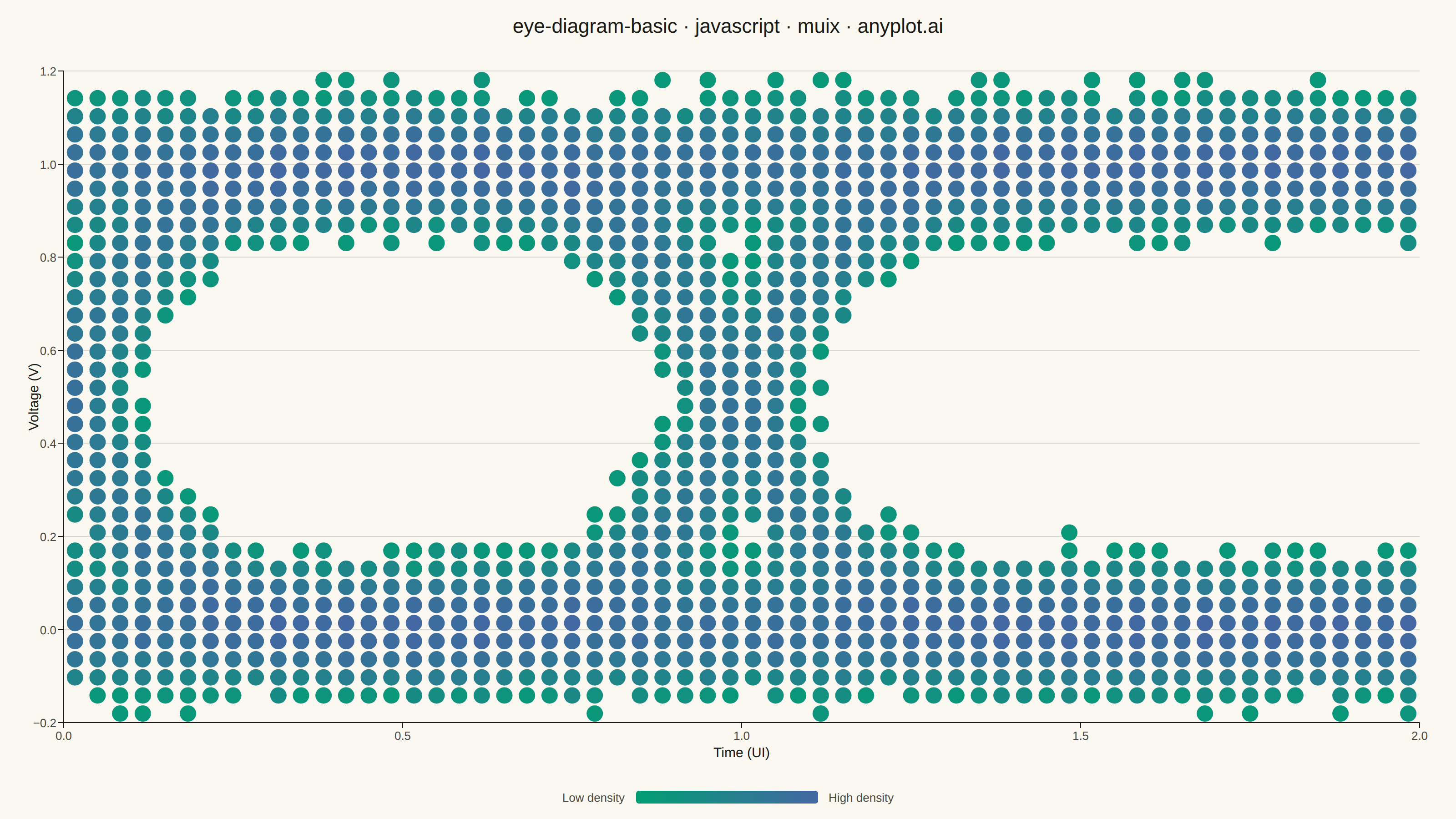
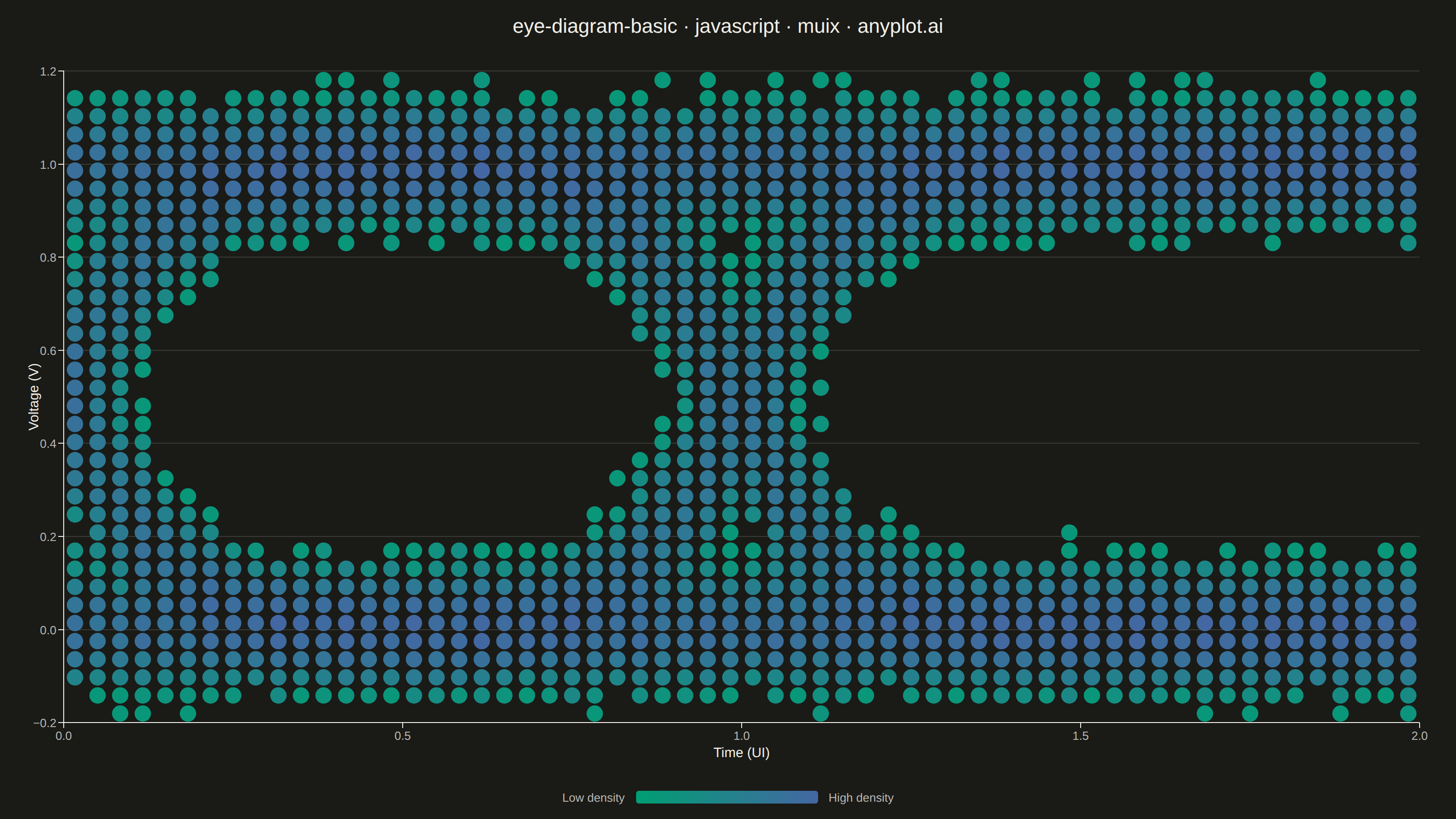
An eye diagram visualizes signal integrity by overlaying many periods of a digital signal onto a single time window spanning 1-2 unit intervals (UI). The overlapping traces form a characteristic eye-shaped opening whose height, width, and clarity reveal signal quality metrics such as jitter, noise, and inter-symbol interference (ISI). A wide-open eye indicates clean signal transmission, while a closed or blurred eye signals degradation.
// anyplot.ai
// eye-diagram-basic: Signal Integrity Eye Diagram
// Library: muix 7.29.1 | JavaScript 22.22.3
// Quality: 84/100 | Created: 2026-06-18
//# anyplot-orientation: landscape
// anyplot.ai
// eye-diagram-basic: Signal Integrity Eye Diagram
// Library: MUI X Charts | React | Node 22
// License: @mui/x-charts — MIT (community). Pro/Premium are out of scope.
// Quality: pending | Created: 2026-06-18

import { ScatterChart } from "@mui/x-charts/ScatterChart";
import Box from "@mui/material/Box";
import Typography from "@mui/material/Typography";

const t = window.ANYPLOT_TOKENS;

// Seeded LCG for reproducible data generation
let _s = 42;
function rand(): number {
  _s = (Math.imul(1664525, _s) + 1013904223) >>> 0;
  return _s / 0x100000000;
}
function randn(): number {
  const u = rand() || 1e-10;
  return Math.sqrt(-2 * Math.log(u)) * Math.cos(2 * Math.PI * rand());
}

// NRZ eye diagram: 300 overlaid traces, each 2 UI long, 200 samples per trace
const N_TRACES = 300;
const N_SAMPLES = 200;

function sigm(x: number): number {
  return 1 / (1 + Math.exp(-12 * x));
}

// Generate raw trace points: sigmoid transitions + random jitter + Gaussian noise
const rawPts: Array<{ x: number; y: number }> = [];
for (let i = 0; i < N_TRACES; i++) {
  const b0 = rand() > 0.5 ? 1 : 0;
  const b1 = rand() > 0.5 ? 1 : 0;
  const b2 = rand() > 0.5 ? 1 : 0;
  const j0 = randn() * 0.03;
  const j1 = randn() * 0.03;
  for (let s = 0; s < N_SAMPLES; s++) {
    const time = (s / (N_SAMPLES - 1)) * 2;
    const voltage =
      b0 +
      (b1 - b0) * sigm(time - j0) +
      (b2 - b1) * sigm(time - 1 - j1) +
      randn() * 0.05;
    rawPts.push({ x: time, y: voltage });
  }
}

// Bin all trace points into a 2D density grid (time × voltage)
const TB = 60;
const VB = 36;
const V0 = -0.2;
const V1 = 1.2;
const grid = new Int32Array(TB * VB);
for (const p of rawPts) {
  if (p.y < V0 || p.y > V1) continue;
  const ti = Math.min(Math.floor((p.x / 2) * TB), TB - 1);
  const vi = Math.min(Math.floor(((p.y - V0) / (V1 - V0)) * VB), VB - 1);
  if (ti >= 0 && vi >= 0) grid[ti * VB + vi]++;
}

// Convert non-zero cells to scatter data with log-density for color mapping
const eyeData: Array<{ id: number; x: number; y: number; z: number }> = [];
let maxZ = 0;
for (let ti = 0; ti < TB; ti++) {
  for (let vi = 0; vi < VB; vi++) {
    const d = grid[ti * VB + vi];
    if (d > 0) {
      const z = Math.log(d + 1);
      if (z > maxZ) maxZ = z;
      eyeData.push({
        id: ti * VB + vi,
        x: ((ti + 0.5) / TB) * 2,
        y: V0 + ((vi + 0.5) / VB) * (V1 - V0),
        z,
      });
    }
  }
}

const TITLE_H = 52;
const COLORBAR_H = 52;

export default function Chart() {
  const W = window.ANYPLOT_SIZE.width;
  const H = window.ANYPLOT_SIZE.height;
  const chartH = H - TITLE_H - COLORBAR_H;

  return (
    <Box
      width={W}
      height={H}
      sx={{
        background: t.pageBg,
        display: "flex",
        flexDirection: "column",
        overflow: "hidden",
      }}
    >
      <Typography
        sx={{
          fontSize: "22px",
          fontWeight: 500,
          color: t.ink,
          px: "32px",
          pt: "16px",
          pb: "4px",
          lineHeight: 1.2,
          textAlign: "center",
        }}
      >
        eye-diagram-basic · javascript · muix · anyplot.ai
      </Typography>
      <ScatterChart
        width={W}
        height={chartH}
        skipAnimation
        margin={{ left: 70, right: 40, top: 20, bottom: 60 }}
        grid={{ vertical: false, horizontal: true }}
        zAxis={[
          {
            id: "density",
            min: 0,
            max: maxZ,
            colorMap: {
              type: "continuous",
              min: 0,
              max: maxZ,
              color: [t.seq[0], t.seq[1]] as [string, string],
            },
          },
        ]}
        series={[
          {
            data: eyeData,
            markerSize: 9,
            zAxisId: "density",
          },
        ]}
        xAxis={[
          {
            label: "Time (UI)",
            min: 0,
            max: 2,
            tickNumber: 5,
            labelStyle: { fontSize: 15, fontWeight: 500, fill: t.ink },
            tickLabelStyle: { fontSize: 13, fill: t.inkSoft },
          },
        ]}
        yAxis={[
          {
            label: "Voltage (V)",
            min: V0,
            max: V1,
            tickNumber: 7,
            labelStyle: { fontSize: 15, fontWeight: 500, fill: t.ink },
            tickLabelStyle: { fontSize: 13, fill: t.inkSoft },
          },
        ]}
      />
      {/* Density scale colorbar */}
      <Box
        sx={{
          display: "flex",
          alignItems: "center",
          justifyContent: "center",
          gap: "12px",
          pb: "14px",
        }}
      >
        <Typography sx={{ fontSize: "13px", color: t.inkSoft }}>
          Low density
        </Typography>
        <Box
          sx={{
            width: 200,
            height: 14,
            borderRadius: "3px",
            background: `linear-gradient(to right, ${t.seq[0]}, ${t.seq[1]})`,
          }}
        />
        <Typography sx={{ fontSize: "13px", color: t.inkSoft }}>
          High density
        </Typography>
      </Box>
    </Box>
  );
}
Runnable source as JSON, for any HTTP client: https://api.anyplot.ai/specs/eye-diagram-basic/muix/code. Any spec id and library id listed in llms-full.txt fit the same URL shape; every URL below is complete and callable.
{
  "spec_id": "eye-diagram-basic",
  "language": "javascript",
  "library": "muix",
  "page": "https://anyplot.ai/eye-diagram-basic/javascript/muix",
  "hub": "https://anyplot.ai/eye-diagram-basic",
  "code_json": "https://api.anyplot.ai/specs/eye-diagram-basic/muix/code",
  "spec_json": "https://api.anyplot.ai/specs/eye-diagram-basic",
  "render_light_png": "https://storage.googleapis.com/anyplot-images/plots/eye-diagram-basic/javascript/muix/plot-light.png",
  "render_dark_png": "https://storage.googleapis.com/anyplot-images/plots/eye-diagram-basic/javascript/muix/plot-dark.png",
  "interactive_light_html": "https://storage.googleapis.com/anyplot-images/plots/eye-diagram-basic/javascript/muix/plot-light.html",
  "interactive_dark_html": "https://storage.googleapis.com/anyplot-images/plots/eye-diagram-basic/javascript/muix/plot-dark.html",
  "quality_score": 84.0,
  "license": "MIT",
  "guide": "https://anyplot.ai/llms.txt"
}
Part of Signal Integrity Eye Diagram on anyplot.ai.