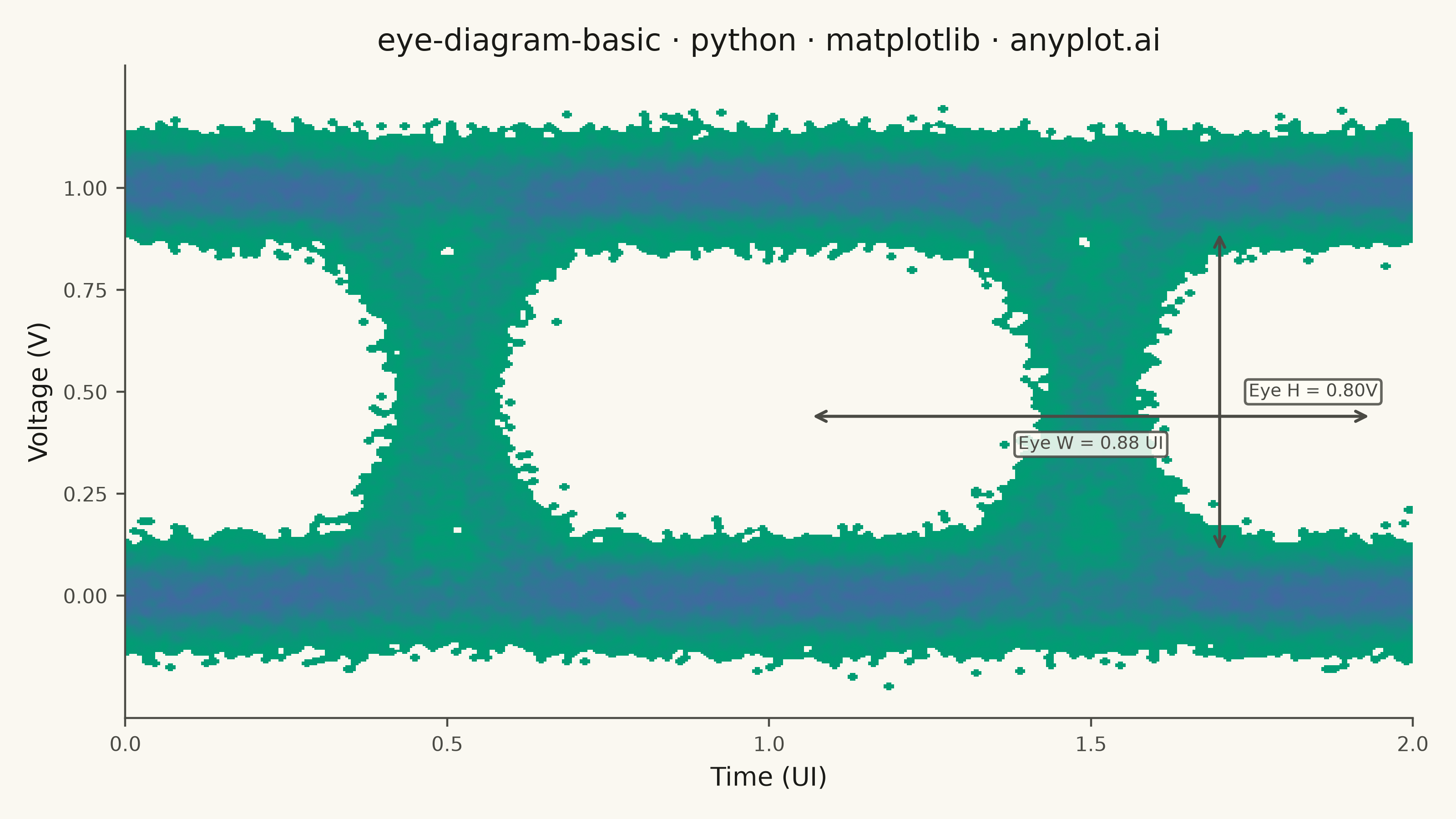
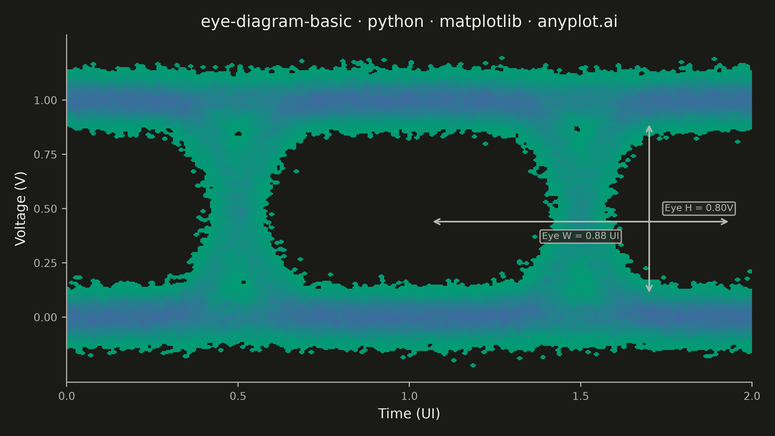
Signal Integrity Eye Diagram — Matplotlib

An eye diagram visualizes signal integrity by overlaying many periods of a digital signal onto a single time window spanning 1-2 unit intervals (UI). The overlapping traces form a characteristic eye-shaped opening whose height, width, and clarity reveal signal quality metrics such as jitter, noise, and inter-symbol interference (ISI). A wide-open eye indicates clean signal transmission, while a closed or blurred eye signals degradation.

Signal Integrity Eye Diagram rendered with Matplotlib

Python source (Matplotlib)

""" anyplot.ai
eye-diagram-basic: Signal Integrity Eye Diagram
Library: matplotlib 3.11.0 | Python 3.13.13
Quality: 90/100 | Updated: 2026-06-18
"""

import os

import matplotlib.pyplot as plt
import numpy as np
from matplotlib.colors import LinearSegmentedColormap
from scipy.ndimage import gaussian_filter


# Theme tokens (Imprint palette, theme-adaptive chrome)
THEME = os.getenv("ANYPLOT_THEME", "light")
PAGE_BG = "#FAF8F1" if THEME == "light" else "#1A1A17"
ELEVATED_BG = "#FFFDF6" if THEME == "light" else "#242420"
INK = "#1A1A17" if THEME == "light" else "#F0EFE8"
INK_SOFT = "#4A4A44" if THEME == "light" else "#B8B7B0"

# Imprint sequential colormap — 3-stop green→cyan→blue for richer visual depth
imprint_seq = LinearSegmentedColormap.from_list("imprint_seq", ["#009E73", "#2ABCCD", "#4467A3"])
imprint_seq.set_bad(color=PAGE_BG)

# Data — simulated NRZ signal with controlled noise and jitter
np.random.seed(42)

n_traces = 400
samples_per_ui = 150
n_bits = 3
noise_sigma = 0.05
jitter_sigma = 0.03

bit_sequences = np.random.randint(0, 2, (n_traces, n_bits + 2))

all_time = []
all_voltage = []

for i in range(n_traces):
    bits = bit_sequences[i]
    t_full = np.linspace(-1, n_bits + 1, (n_bits + 2) * samples_per_ui)
    signal = np.zeros_like(t_full)

    for b in range(n_bits + 2):
        signal += bits[b] * (1 / (1 + np.exp(-20 * (t_full - b + 0.5))))
        if b > 0:
            signal -= bits[b - 1] * (1 / (1 + np.exp(-20 * (t_full - b + 0.5))))

    t_jittered = t_full + np.random.normal(0, jitter_sigma, len(t_full))
    noise = np.random.normal(0, noise_sigma, len(t_full))
    signal_noisy = signal + noise

    mask = (t_jittered >= 0) & (t_jittered <= 2)
    all_time.extend(t_jittered[mask])
    all_voltage.extend(signal_noisy[mask])

all_time = np.array(all_time)
all_voltage = np.array(all_voltage)

# 2D density histogram with Gaussian smoothing for crisp rendering
h, xedges, yedges = np.histogram2d(all_time, all_voltage, bins=[500, 340], range=[[0, 2], [-0.3, 1.3]])
h_smooth = gaussian_filter(np.log1p(h.T), sigma=1.2)
h_masked = np.ma.masked_where(h_smooth < 0.01, h_smooth)

# Eye measurements — 2-sigma approximation from simulation parameters
eye_height = 1.0 - 4 * noise_sigma  # ~0.80V
eye_width = 1.0 - 4 * jitter_sigma  # ~0.88 UI

# Plot
fig, ax = plt.subplots(figsize=(8, 4.5), dpi=400, facecolor=PAGE_BG)
ax.set_facecolor(PAGE_BG)

im = ax.imshow(
    h_masked, origin="lower", aspect="auto", extent=[0, 2, -0.3, 1.3], cmap=imprint_seq, interpolation="bilinear"
)

# Nominal signal level reference lines at 0 V and 1 V
for ref_v in (0.0, 1.0):
    ax.axhline(ref_v, color=INK_SOFT, linestyle="--", linewidth=0.8, alpha=0.40)

# Faint y-axis grid to aid voltage estimation (drawn above heatmap)
ax.yaxis.grid(True, alpha=0.10, linewidth=0.6, color=INK)

# Eye height annotation — vertical arrow in the second eye opening (shifted left from edge)
t_annot = 1.62
ax.annotate(
    "", xy=(t_annot, 0.10), xytext=(t_annot, 0.90), arrowprops={"arrowstyle": "<->", "color": INK_SOFT, "lw": 1.2}
)
ax.text(
    1.67,
    0.50,
    f"Eye H = {eye_height:.2f}V",
    fontsize=7,
    color=INK_SOFT,
    va="center",
    bbox={"facecolor": ELEVATED_BG, "edgecolor": INK_SOFT, "alpha": 0.85, "boxstyle": "round,pad=0.2"},
)

# Eye width annotation — horizontal arrow across second eye opening at mid-voltage
t_left = 1.0 + (1.0 - eye_width) / 2
t_right = 2.0 - (1.0 - eye_width) / 2
ax.annotate(
    "", xy=(t_left, 0.44), xytext=(t_right, 0.44), arrowprops={"arrowstyle": "<->", "color": INK_SOFT, "lw": 1.2}
)
ax.text(
    1.50,
    0.36,
    f"Eye W = {eye_width:.2f} UI",
    fontsize=7,
    color=INK_SOFT,
    ha="center",
    bbox={"facecolor": ELEVATED_BG, "edgecolor": INK_SOFT, "alpha": 0.85, "boxstyle": "round,pad=0.2"},
)

# Colorbar — trace density scale (primary matplotlib heatmap feature)
cbar = fig.colorbar(im, ax=ax, shrink=0.75, pad=0.02, aspect=25)
cbar.set_label("Trace density (log)", fontsize=8, color=INK_SOFT)
cbar.ax.tick_params(labelsize=7, colors=INK_SOFT, labelcolor=INK_SOFT)
cbar.outline.set_edgecolor(INK_SOFT)
cbar.ax.set_facecolor(PAGE_BG)

# Style
title = "eye-diagram-basic · python · matplotlib · anyplot.ai"
ax.set_xlabel("Time (UI)", fontsize=10, color=INK)
ax.set_ylabel("Voltage (V)", fontsize=10, color=INK)
ax.set_title(title, fontsize=12, fontweight="medium", color=INK)
ax.tick_params(axis="both", labelsize=8, colors=INK_SOFT)

ax.set_xticks([0, 0.5, 1.0, 1.5, 2.0])
ax.set_yticks([0, 0.25, 0.5, 0.75, 1.0])

ax.spines["top"].set_visible(False)
ax.spines["right"].set_visible(False)
for s in ("left", "bottom"):
    ax.spines[s].set_color(INK_SOFT)

plt.tight_layout()

# Save — no bbox_inches to preserve exact 3200×1800 canvas
plt.savefig(f"plot-{THEME}.png", dpi=400, facecolor=PAGE_BG)
plt.close()

Part of Signal Integrity Eye Diagram on anyplot.ai.

Signal Integrity Eye Diagram — Matplotlib

Python source (Matplotlib)

Other implementations