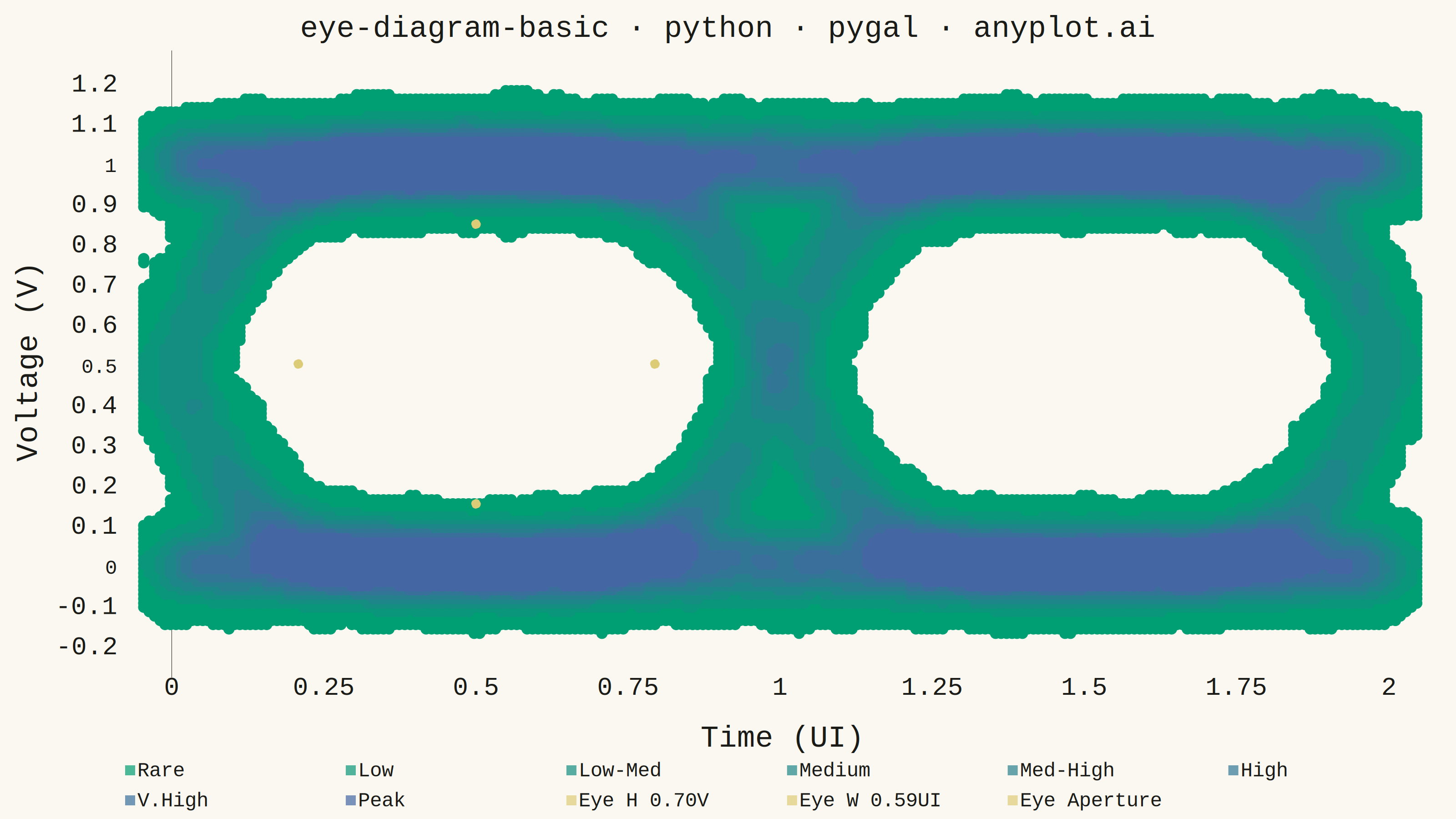
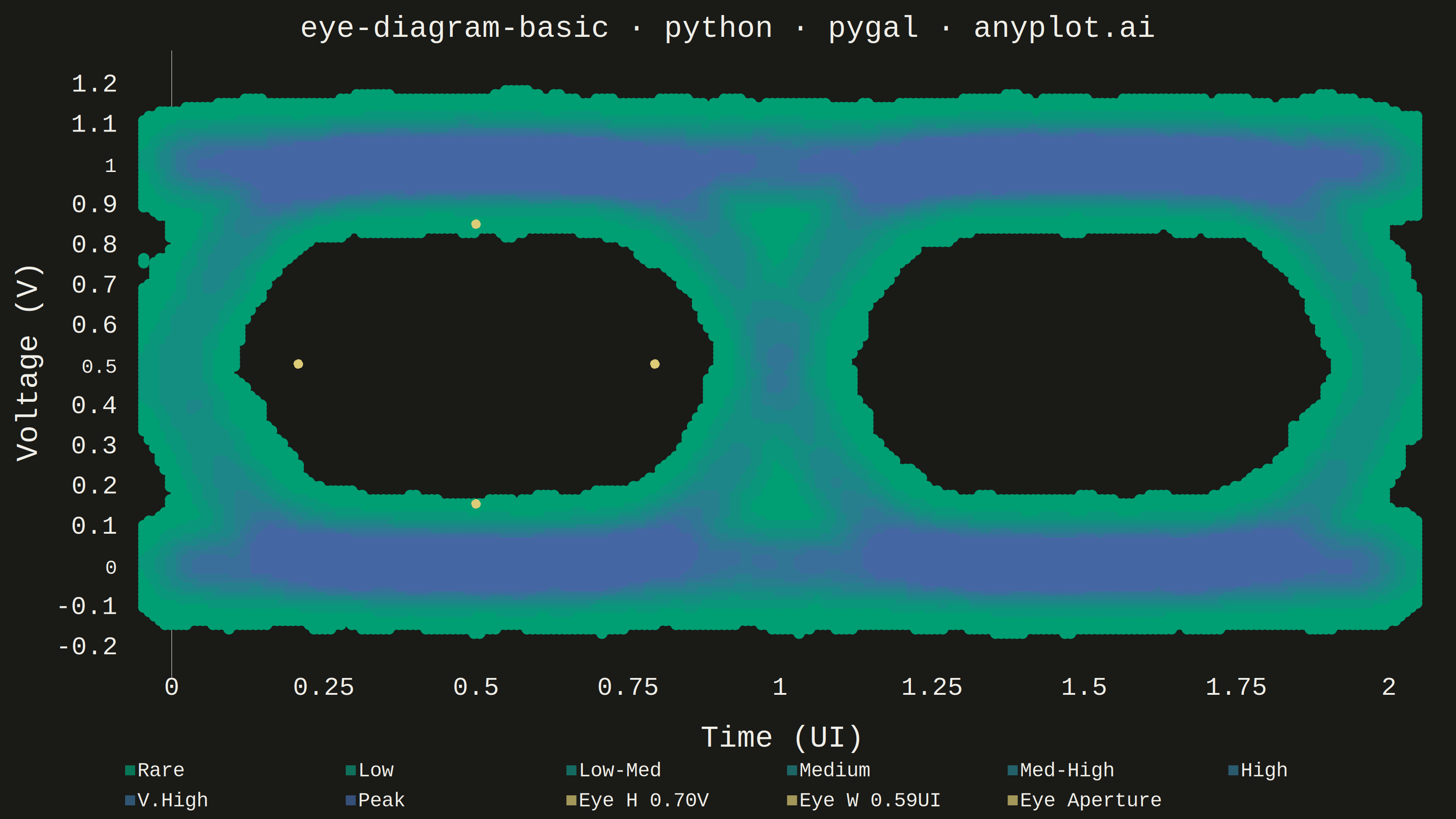
An eye diagram visualizes signal integrity by overlaying many periods of a digital signal onto a single time window spanning 1-2 unit intervals (UI). The overlapping traces form a characteristic eye-shaped opening whose height, width, and clarity reveal signal quality metrics such as jitter, noise, and inter-symbol interference (ISI). A wide-open eye indicates clean signal transmission, while a closed or blurred eye signals degradation.
""" anyplot.ai
eye-diagram-basic: Signal Integrity Eye Diagram
Library: pygal 3.1.0 | Python 3.13.13
Quality: 86/100 | Updated: 2026-06-18
"""

import importlib
import os
import sys

import numpy as np


# Import pygal avoiding name collision with this filename
_cwd = sys.path[0]
sys.path[:] = [p for p in sys.path if p != _cwd]
pygal = importlib.import_module("pygal")
Style = importlib.import_module("pygal.style").Style
sys.path.insert(0, _cwd)

# Theme tokens (Imprint palette)
THEME = os.getenv("ANYPLOT_THEME", "light")
PAGE_BG = "#FAF8F1" if THEME == "light" else "#1A1A17"
INK = "#1A1A17" if THEME == "light" else "#F0EFE8"
INK_MUTED = "#6B6A63" if THEME == "light" else "#A8A79F"
ANYPLOT_AMBER = "#DDCC77"  # annotation / measurement marker

# Imprint sequential colormap: brand green → blue for density heatmap
# imprint_seq: #009E73 (low density) → #4467A3 (high density)
N_BANDS = 8
_seq_t = np.linspace(0, 1, N_BANDS)
_seq_start = np.array([0x00, 0x9E, 0x73])  # #009E73
_seq_end = np.array([0x44, 0x67, 0xA3])  # #4467A3
density_colors = tuple(
    "#" + "".join(f"{int(round(c)):02X}" for c in (_seq_start + (_seq_end - _seq_start) * t)) for t in _seq_t
)
band_names = ["Rare", "Low", "Low-Med", "Medium", "Med-High", "High", "V.High", "Peak"]

# Data — simulated NRZ eye diagram
np.random.seed(42)

n_traces = 400
samples_per_ui = 200
total_samples = samples_per_ui * 2  # 2 UI window
time_ui = np.linspace(0, 2, total_samples)
transition_width = 0.07  # UI, controls bandwidth-limited rise/fall

all_voltages = []
for _ in range(n_traces):
    bits = np.random.randint(0, 2, 6)
    extended_time = np.linspace(-1, 3, samples_per_ui * 4)
    voltage = np.zeros_like(extended_time)

    for bit_idx in range(1, len(bits)):
        boundary = bit_idx - 2
        voltage += (bits[bit_idx] - bits[bit_idx - 1]) / (1.0 + np.exp(-(extended_time - boundary) / transition_width))
    voltage += bits[0]
    voltage = np.clip(voltage, -0.2, 1.2)

    mask = (extended_time >= 0) & (extended_time <= 2)
    trace_voltage = voltage[mask][:total_samples]

    trace_voltage = trace_voltage + np.random.normal(0, 0.05, len(trace_voltage))
    jittered_time = time_ui + np.random.normal(0, 0.03)
    all_voltages.append((jittered_time, trace_voltage))

# Build 2D density histogram
n_xbins, n_ybins = 240, 140
x_edges = np.linspace(-0.05, 2.05, n_xbins + 1)
y_edges = np.linspace(-0.25, 1.25, n_ybins + 1)
density = np.zeros((n_ybins, n_xbins))

for jittered_time, trace_voltage in all_voltages:
    xi = ((jittered_time - x_edges[0]) / (x_edges[-1] - x_edges[0]) * n_xbins).astype(int)
    yi = ((trace_voltage - y_edges[0]) / (y_edges[-1] - y_edges[0]) * n_ybins).astype(int)
    valid = (xi >= 0) & (xi < n_xbins) & (yi >= 0) & (yi < n_ybins)
    for x, y in zip(xi[valid], yi[valid], strict=True):
        density[y, x] += 1

# 4-pass 3×3 box filter for smoother density gradients
for _ in range(4):
    padded = np.pad(density, 1, mode="edge")
    density = (
        padded[:-2, :-2]
        + padded[:-2, 1:-1]
        + padded[:-2, 2:]
        + padded[1:-1, :-2]
        + padded[1:-1, 1:-1]
        + padded[1:-1, 2:]
        + padded[2:, :-2]
        + padded[2:, 1:-1]
        + padded[2:, 2:]
    ) / 9.0

max_density = density.max()

# Eye opening metrics for annotations
center_col = int(0.5 * n_xbins / 2.1)
col_density = density[:, center_col]
y_centers = (y_edges[:-1] + y_edges[1:]) / 2

threshold = max_density * 0.15
low_indices = np.where(col_density < threshold)[0]
eye_region = low_indices[(y_centers[low_indices] > 0.15) & (y_centers[low_indices] < 0.85)]
if len(eye_region) > 2:
    eye_bottom = y_centers[eye_region[0]]
    eye_top = y_centers[eye_region[-1]]
    eye_height = round(eye_top - eye_bottom, 3)
else:
    eye_bottom, eye_top, eye_height = 0.2, 0.8, 0.6

mid_row = int((0.5 - y_edges[0]) / (y_edges[-1] - y_edges[0]) * n_ybins)
mid_row = np.clip(mid_row, 0, n_ybins - 1)
row_density = density[mid_row, :]
x_centers = (x_edges[:-1] + x_edges[1:]) / 2
low_x_indices = np.where(row_density < threshold)[0]
eye_x_region = low_x_indices[(x_centers[low_x_indices] > 0.2) & (x_centers[low_x_indices] < 0.8)]
if len(eye_x_region) > 2:
    eye_left = x_centers[eye_x_region[0]]
    eye_right = x_centers[eye_x_region[-1]]
    eye_width = round(eye_right - eye_left, 3)
else:
    eye_left, eye_right, eye_width = 0.3, 0.7, 0.4

# Assign density cells to Imprint sequential color bands
band_data = [[] for _ in range(N_BANDS)]
for yi in range(n_ybins):
    for xi in range(n_xbins):
        val = density[yi, xi]
        if val < 0.2:
            continue
        t = min(0.999, val / (max_density * 0.55))
        band_idx = min(int(t * N_BANDS), N_BANDS - 1)
        x_center = round((x_edges[xi] + x_edges[xi + 1]) / 2, 3)
        y_center = round((y_edges[yi] + y_edges[yi + 1]) / 2, 3)
        pct = round(val / max_density * 100, 1)
        band_data[band_idx].append(
            {"value": (x_center, y_center), "label": f"{x_center:.2f} UI, {y_center:.3f} V — {pct}%"}
        )

# Eye measurement annotation series — amber for high visibility against density field
eye_height_line = [
    {"value": (0.5, round(eye_bottom, 3)), "label": f"Eye Height: {eye_height:.3f} V"},
    {"value": (0.5, round(eye_top, 3)), "label": f"Eye Height: {eye_height:.3f} V"},
]
eye_width_line = [
    {"value": (round(eye_left, 3), 0.5), "label": f"Eye Width: {eye_width:.3f} UI"},
    {"value": (round(eye_right, 3), 0.5), "label": f"Eye Width: {eye_width:.3f} UI"},
]
# Rectangle bounding the eye aperture — closes the box so the open eye is the clear focal point
eye_aperture_box = [
    {"value": (round(eye_left, 3), round(eye_bottom, 3)), "label": "Eye Aperture"},
    {"value": (round(eye_left, 3), round(eye_top, 3)), "label": "Eye Aperture"},
    {"value": (round(eye_right, 3), round(eye_top, 3)), "label": "Eye Aperture"},
    {"value": (round(eye_right, 3), round(eye_bottom, 3)), "label": "Eye Aperture"},
    {"value": (round(eye_left, 3), round(eye_bottom, 3)), "label": "Eye Aperture"},
]

# pygal Style — theme-adaptive with Imprint sequential palette
custom_style = Style(
    background=PAGE_BG,
    plot_background=PAGE_BG,
    foreground=INK,
    foreground_strong=INK,
    foreground_subtle=INK_MUTED,
    colors=density_colors + (ANYPLOT_AMBER, ANYPLOT_AMBER, ANYPLOT_AMBER),
    title_font_size=66,
    label_font_size=56,
    major_label_font_size=44,
    legend_font_size=44,
    value_font_size=36,
    tooltip_font_size=32,
    stroke_width=0,
    font_family="'Courier New', monospace",
    title_font_family="'Courier New', monospace",
    label_font_family="'Courier New', monospace",
    legend_font_family="'Courier New', monospace",
    value_font_family="'Courier New', monospace",
)

# XY scatter chart — 3200×1800 landscape canvas
chart = pygal.XY(
    width=3200,
    height=1800,
    style=custom_style,
    title="eye-diagram-basic · python · pygal · anyplot.ai",
    x_title="Time (UI)",
    y_title="Voltage (V)",
    stroke=False,
    dots_size=12,
    show_legend=True,
    legend_at_bottom=True,
    legend_at_bottom_columns=6,
    legend_box_size=22,
    show_x_guides=False,
    show_y_guides=False,
    x_labels=[0.0, 0.25, 0.5, 0.75, 1.0, 1.25, 1.5, 1.75, 2.0],
    range=(-0.25, 1.25),
    x_label_rotation=0,
    truncate_label=-1,
    print_values=False,
    show_dots=True,
    margin=30,
    margin_bottom=100,
    spacing=15,
    js=[],
)

for i in range(N_BANDS):
    chart.add(band_names[i], band_data[i] if band_data[i] else [], allow_interruptions=True)

chart.add(
    f"Eye H {eye_height:.2f}V",
    eye_height_line,
    stroke=True,
    show_dots=True,
    dots_size=10,
    stroke_style={"width": 4, "dasharray": "10, 5"},
    allow_interruptions=False,
)
chart.add(
    f"Eye W {eye_width:.2f}UI",
    eye_width_line,
    stroke=True,
    show_dots=True,
    dots_size=10,
    stroke_style={"width": 4, "dasharray": "10, 5"},
    allow_interruptions=False,
)
chart.add(
    "Eye Aperture",
    eye_aperture_box,
    stroke=True,
    show_dots=False,
    stroke_style={"width": 3, "dasharray": "6, 4"},
    allow_interruptions=False,
)

# Save PNG and interactive HTML
chart.render_to_png(f"plot-{THEME}.png")

svg_content = chart.render(is_unicode=True)
html_content = f"""<!DOCTYPE html>
<html>
<head>
    <meta charset="utf-8">
    <title>eye-diagram-basic · python · pygal · anyplot.ai</title>
    <style>
        body {{ margin: 0; display: flex; justify-content: center; align-items: center;
               min-height: 100vh; background: {PAGE_BG}; }}
        .chart {{ max-width: 100%; height: auto; }}
    </style>
</head>
<body>
    <figure class="chart">
        {svg_content}
    </figure>
</body>
</html>
"""

with open(f"plot-{THEME}.html", "w", encoding="utf-8") as fout:
    fout.write(html_content)
Runnable source as JSON, for any HTTP client: https://api.anyplot.ai/specs/eye-diagram-basic/pygal/code. Any spec id and library id listed in llms-full.txt fit the same URL shape; every URL below is complete and callable.
{
  "spec_id": "eye-diagram-basic",
  "language": "python",
  "library": "pygal",
  "page": "https://anyplot.ai/eye-diagram-basic/python/pygal",
  "hub": "https://anyplot.ai/eye-diagram-basic",
  "code_json": "https://api.anyplot.ai/specs/eye-diagram-basic/pygal/code",
  "spec_json": "https://api.anyplot.ai/specs/eye-diagram-basic",
  "render_light_png": "https://storage.googleapis.com/anyplot-images/plots/eye-diagram-basic/python/pygal/plot-light.png",
  "render_dark_png": "https://storage.googleapis.com/anyplot-images/plots/eye-diagram-basic/python/pygal/plot-dark.png",
  "interactive_light_html": "https://storage.googleapis.com/anyplot-images/plots/eye-diagram-basic/python/pygal/plot-light.html",
  "interactive_dark_html": "https://storage.googleapis.com/anyplot-images/plots/eye-diagram-basic/python/pygal/plot-dark.html",
  "quality_score": 86.0,
  "license": "MIT",
  "guide": "https://anyplot.ai/llms.txt"
}
Part of Signal Integrity Eye Diagram on anyplot.ai.