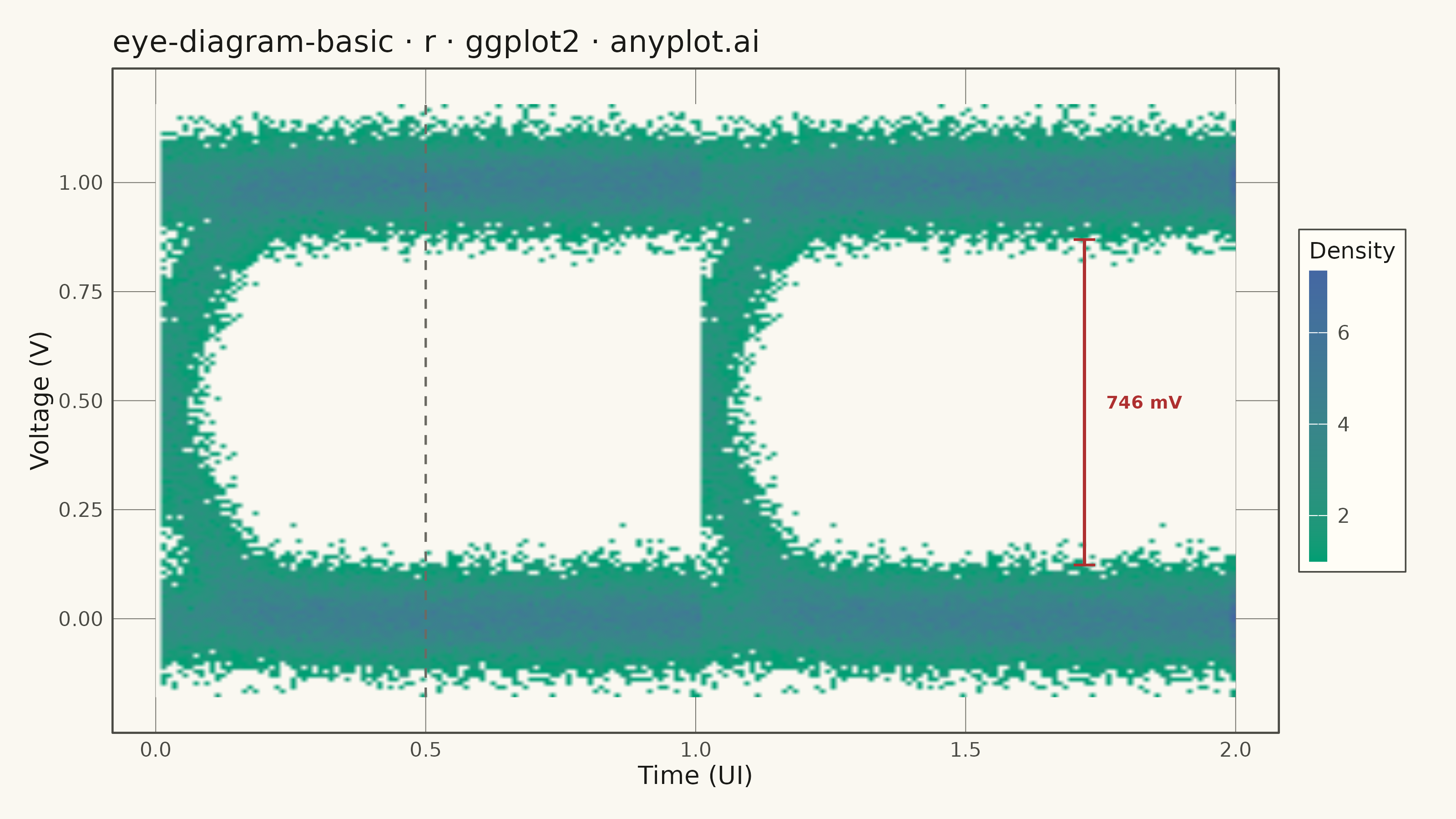
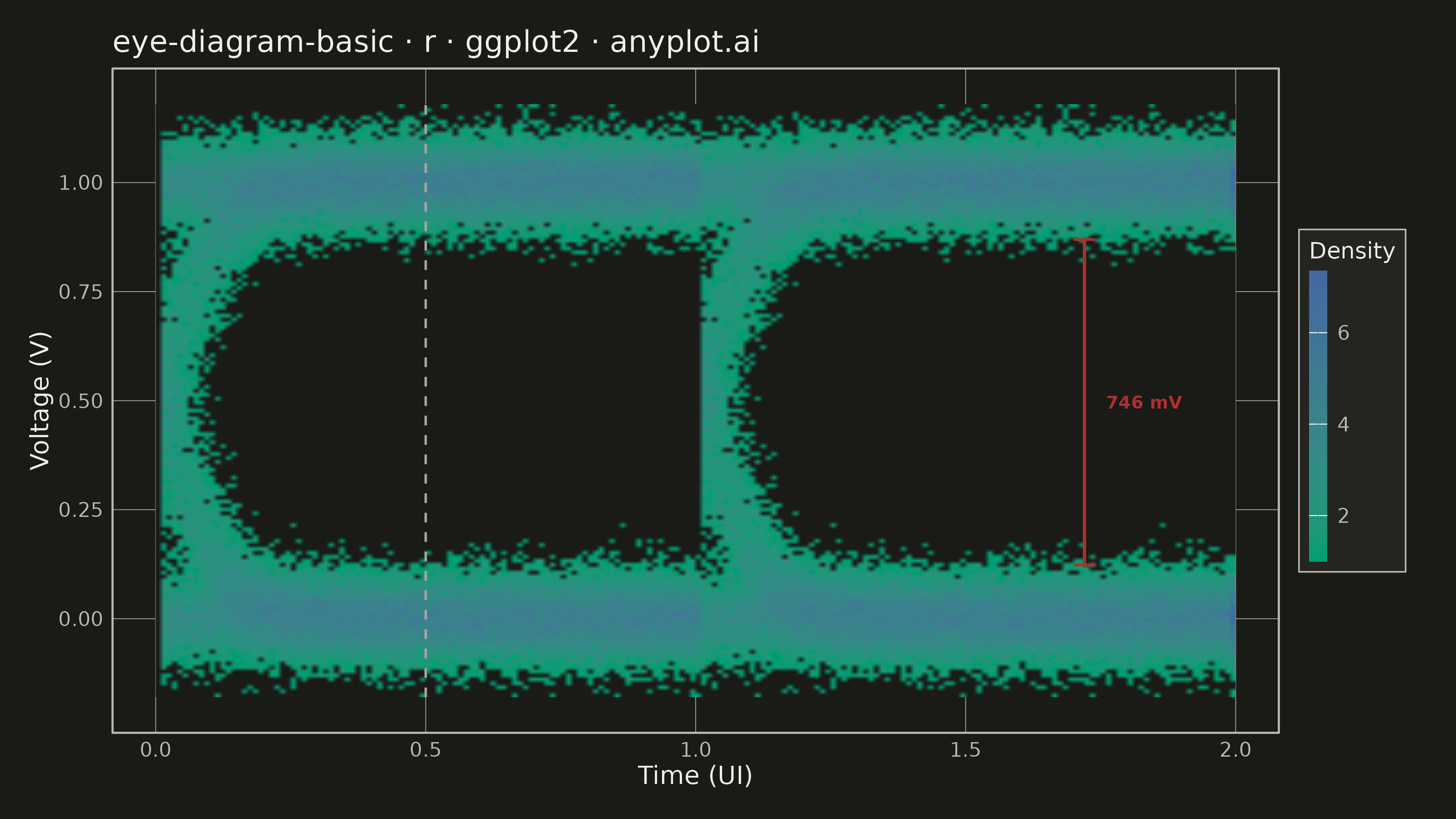
An eye diagram visualizes signal integrity by overlaying many periods of a digital signal onto a single time window spanning 1-2 unit intervals (UI). The overlapping traces form a characteristic eye-shaped opening whose height, width, and clarity reveal signal quality metrics such as jitter, noise, and inter-symbol interference (ISI). A wide-open eye indicates clean signal transmission, while a closed or blurred eye signals degradation.
#' anyplot.ai
#' eye-diagram-basic: Signal Integrity Eye Diagram
#' Library: ggplot2 3.5.1 | R 4.4.1
#' Quality: 92/100 | Created: 2026-06-18

library(ggplot2)
library(ragg)

set.seed(42)

# Theme tokens (Imprint palette, theme-adaptive chrome)
THEME       <- Sys.getenv("ANYPLOT_THEME", "light")
PAGE_BG     <- if (THEME == "light") "#FAF8F1" else "#1A1A17"
ELEVATED_BG <- if (THEME == "light") "#FFFDF6" else "#242420"
INK         <- if (THEME == "light") "#1A1A17" else "#F0EFE8"
INK_SOFT    <- if (THEME == "light") "#4A4A44" else "#B8B7B0"
INK_MUTED   <- if (THEME == "light") "#6B6A63" else "#A8A79F"

# NRZ simulation parameters
n_bits       <- 600
samp_per_ui  <- 100
noise_sigma  <- 0.05   # Gaussian noise (5% of amplitude)
jitter_sigma <- 0.03   # Timing jitter std dev (3% of UI)
sigmoid_k    <- 18     # Bandwidth-limiting sharpness

# Random bit stream and per-transition jitter
bits       <- sample(c(0L, 1L), n_bits, replace = TRUE)
jitter_raw <- rnorm(n_bits - 1L, 0.0, jitter_sigma)
j_arr      <- c(0.0, jitter_raw)

# Vectorized waveform generation with sigmoid transitions and jitter
n_total   <- n_bits * samp_per_ui
t_all     <- (seq_len(n_total) - 0.5) / samp_per_ui
bit_idx   <- pmin(as.integer(floor(t_all)) + 1L, n_bits)
t_within  <- t_all - floor(t_all)
prev_bits <- c(bits[1L], bits[-n_bits])
prev_at_t <- prev_bits[bit_idx]
curr_at_t <- bits[bit_idx]
j_vals    <- j_arr[bit_idx]

dt    <- (t_within - j_vals) * sigmoid_k
sig_s <- 1.0 / (1.0 + exp(-dt))
same  <- (prev_at_t == curr_at_t)
rise  <- (!same & curr_at_t > prev_at_t)
v_sig <- ifelse(same, curr_at_t * 1.0, ifelse(rise, sig_s, 1.0 - sig_s))
v_sig <- v_sig + rnorm(n_total, 0.0, noise_sigma)

# Fold waveform into 2-UI eye traces (start at each bit boundary)
window_sz <- 2L * samp_per_ui
n_traces  <- n_bits - 2L
t_axis    <- seq(0.0, 2.0, length.out = window_sz + 1L)[-1L]
start_idx <- (seq_len(n_traces) - 1L) * samp_per_ui + 1L
samp_mat  <- outer(0L:(window_sz - 1L), start_idx, `+`)
eye_df    <- data.frame(
    time    = rep(t_axis, n_traces),
    voltage = v_sig[as.vector(samp_mat)]
)

# Pre-compute 2D density grid: vectorised findInterval + tabulate → geom_raster
n_bins_x <- 200
n_bins_y <- 150
t_breaks <- seq(0.0,  2.0,  length.out = n_bins_x + 1L)
v_breaks <- seq(-0.18, 1.18, length.out = n_bins_y + 1L)
t_mids   <- (t_breaks[-1L] + t_breaks[-length(t_breaks)]) / 2
v_mids   <- (v_breaks[-1L] + v_breaks[-length(v_breaks)]) / 2

t_bin_idx <- pmin(pmax(findInterval(eye_df$time,    t_breaks), 1L), n_bins_x)
v_bin_idx <- pmin(pmax(findInterval(eye_df$voltage, v_breaks), 1L), n_bins_y)
lin_idx   <- (t_bin_idx - 1L) * n_bins_y + v_bin_idx
count_vec <- tabulate(lin_idx, nbins = n_bins_x * n_bins_y)

# Full rectangular grid required for geom_raster interpolation;
# zero-count cells → NA so scale maps them to PAGE_BG (eye opening shows through)
raster_df <- data.frame(
    time    = rep(t_mids, each = n_bins_y),
    voltage = rep(v_mids, times = n_bins_x),
    density = ifelse(count_vec > 0L, sqrt(count_vec), NA_real_)
)

# Estimate eye opening at optimal sampling point (t ≈ 1.5 UI, centre of second eye)
at_center  <- eye_df$time >= 1.40 & eye_df$time <= 1.60
center_v   <- eye_df$voltage[at_center]
low_level  <- center_v[center_v < 0.5]
high_level <- center_v[center_v > 0.5]
eye_lo     <- if (length(low_level)  > 10L) as.numeric(quantile(low_level,  0.995)) else 0.15
eye_hi     <- if (length(high_level) > 10L) as.numeric(quantile(high_level, 0.005)) else 0.85
eye_ht_mv  <- max(0L, round((eye_hi - eye_lo) * 1000L))

plot_title <- "eye-diagram-basic · r · ggplot2 · anyplot.ai"

p <- ggplot(raster_df, aes(x = time, y = voltage)) +
    # Smooth density heatmap via bilinear-interpolated raster (publication-quality)
    geom_raster(aes(fill = density), interpolate = TRUE) +
    # Optimal sampling point (t=0.5, centre of first eye) — vertical dashed reference
    annotate("segment", x = 0.5, xend = 0.5,
             y = min(v_breaks), yend = max(v_breaks),
             color = INK_MUTED, linewidth = 0.45, linetype = "dashed") +
    # Eye height bracket: bracket bar + serif ticks + measurement label
    annotate("segment", x = 1.72, xend = 1.72, y = eye_lo, yend = eye_hi,
             color = "#AE3030", linewidth = 0.6) +
    annotate("segment", x = 1.70, xend = 1.74, y = eye_lo, yend = eye_lo,
             color = "#AE3030", linewidth = 0.5) +
    annotate("segment", x = 1.70, xend = 1.74, y = eye_hi, yend = eye_hi,
             color = "#AE3030", linewidth = 0.5) +
    annotate("text", x = 1.76, y = (eye_lo + eye_hi) / 2,
             label = paste0(eye_ht_mv, " mV"),
             color = "#AE3030", size = 2.5, hjust = 0.0, fontface = "bold") +
    scale_fill_gradient(
        name     = "Density",
        low      = "#009E73",
        high     = "#4467A3",
        na.value = PAGE_BG,
        guide    = guide_colorbar(barwidth = 0.5, barheight = 8)
    ) +
    scale_x_continuous(
        name   = "Time (UI)",
        breaks = c(0.0, 0.5, 1.0, 1.5, 2.0),
        expand = c(0.04, 0.0)
    ) +
    scale_y_continuous(
        name   = "Voltage (V)",
        breaks = c(0.0, 0.25, 0.5, 0.75, 1.0),
        expand = c(0.06, 0.0)
    ) +
    coord_cartesian(clip = "off") +
    labs(title = plot_title) +
    theme_minimal(base_size = 8) +
    theme(
        plot.background   = element_rect(fill = PAGE_BG,     color = PAGE_BG),
        panel.background  = element_rect(fill = PAGE_BG,     color = NA),
        panel.grid.major  = element_line(color = INK_MUTED,  linewidth = 0.15),
        panel.grid.minor  = element_blank(),
        panel.border      = element_rect(fill = NA,          color = INK_SOFT, linewidth = 0.4),
        axis.title        = element_text(color = INK,        size = 10),
        axis.text         = element_text(color = INK_SOFT,   size = 8),
        plot.title        = element_text(color = INK,        size = 12, hjust = 0.0),
        legend.background = element_rect(fill = ELEVATED_BG, color = INK_SOFT, linewidth = 0.3),
        legend.text       = element_text(color = INK_SOFT,   size = 8),
        legend.title      = element_text(color = INK,        size = 9),
        legend.position   = "right",
        plot.margin       = margin(12, 20, 12, 12, "pt")
    )

ggsave(
    filename = sprintf("plot-%s.png", THEME),
    plot     = p,
    device   = ragg::agg_png,
    width    = 8,
    height   = 4.5,
    units    = "in",
    dpi      = 400
)
Runnable source as JSON, for any HTTP client: https://api.anyplot.ai/specs/eye-diagram-basic/ggplot2/code. Any spec id and library id listed in llms-full.txt fit the same URL shape; every URL below is complete and callable.
{
  "spec_id": "eye-diagram-basic",
  "language": "r",
  "library": "ggplot2",
  "page": "https://anyplot.ai/eye-diagram-basic/r/ggplot2",
  "hub": "https://anyplot.ai/eye-diagram-basic",
  "code_json": "https://api.anyplot.ai/specs/eye-diagram-basic/ggplot2/code",
  "spec_json": "https://api.anyplot.ai/specs/eye-diagram-basic",
  "render_light_png": "https://storage.googleapis.com/anyplot-images/plots/eye-diagram-basic/r/ggplot2/plot-light.png",
  "render_dark_png": "https://storage.googleapis.com/anyplot-images/plots/eye-diagram-basic/r/ggplot2/plot-dark.png",
  "quality_score": 92.0,
  "license": "MIT",
  "guide": "https://anyplot.ai/llms.txt"
}
Part of Signal Integrity Eye Diagram on anyplot.ai.