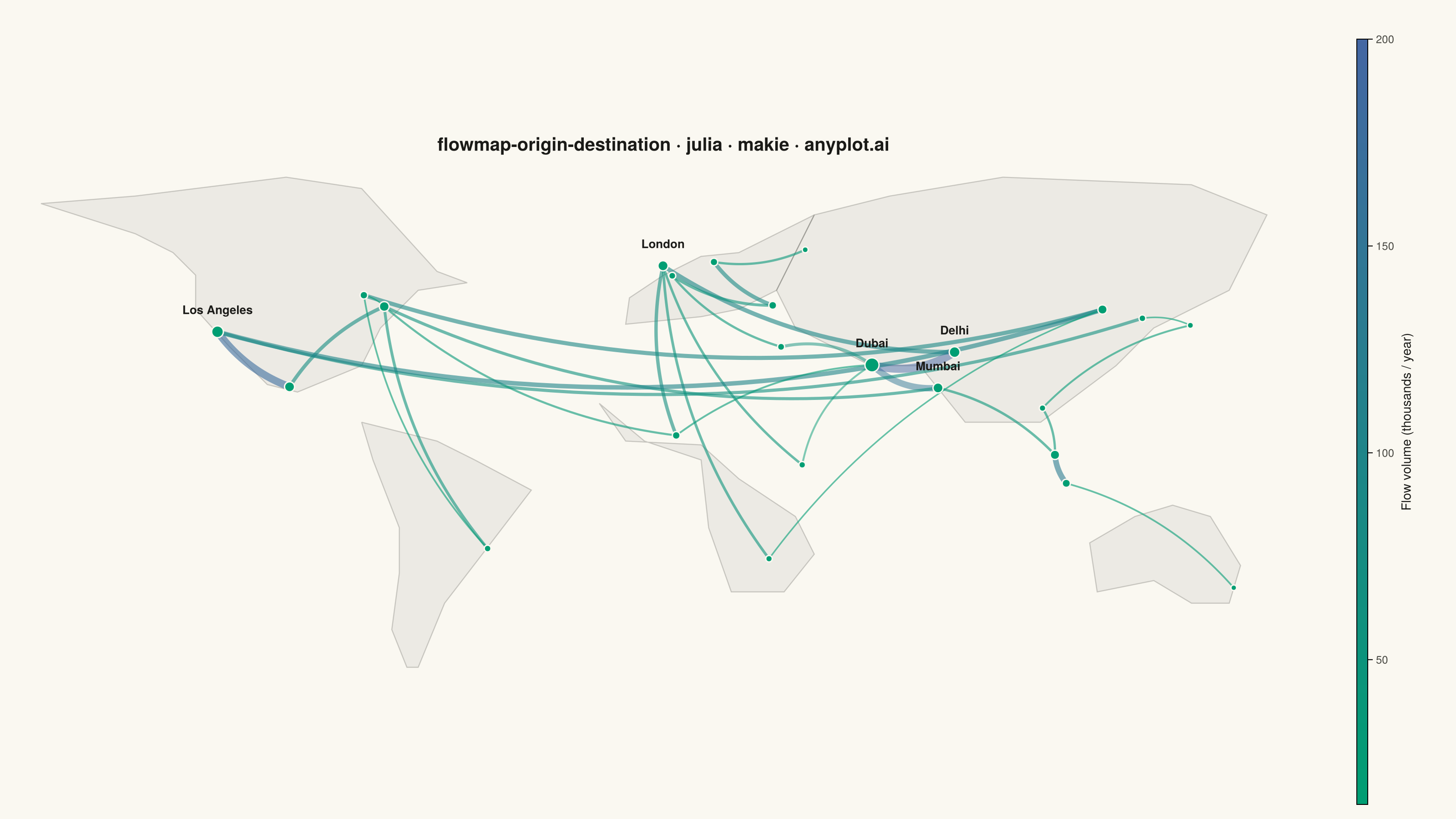
The same plot in 14 other libraries — Python: Altair, Bokeh, lets-plot, Matplotlib, Plotly, plotnine, Pygal, Seaborn; R: ggplot2; JavaScript: Chart.js, D3.js, Apache ECharts, Highcharts, MUI X Charts. Compare all 15 side by side: Origin-Destination Flow Map in Python, R, Julia and JavaScript.
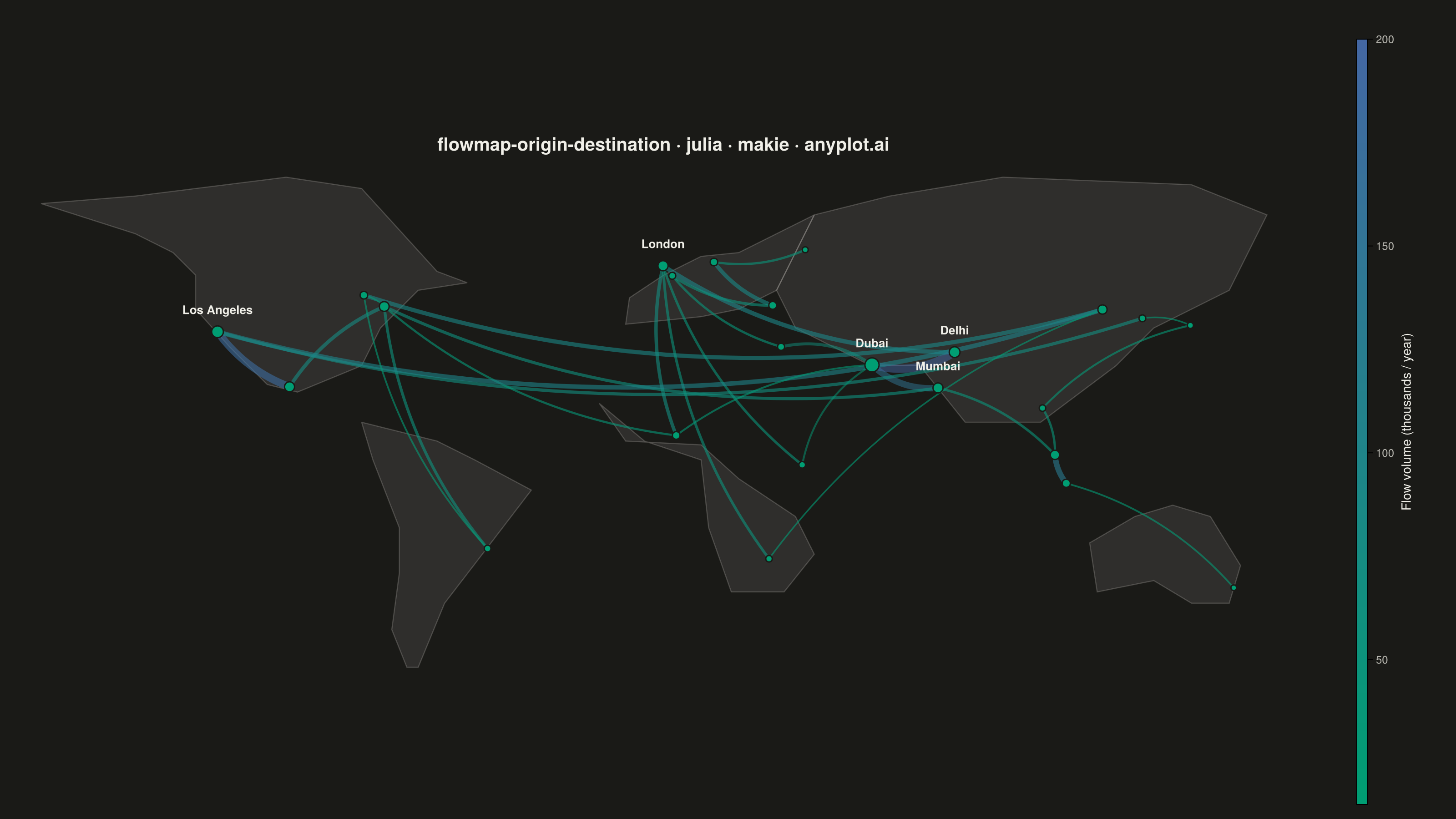
An origin-destination flow map visualizes movement or transfer between geographic locations using curved arcs overlaid on a map. Each arc connects an origin point to a destination point, with line thickness proportional to the flow magnitude. This visualization excels at revealing spatial patterns in migration, trade, or travel data, making it easy to identify major corridors, hub locations, and directional imbalances in movement between places.
# anyplot.ai
# flowmap-origin-destination: Origin-Destination Flow Map
# Library: makie 0.21.9 | Julia 1.11.9
# Quality: 89/100 | Created: 2026-09-02

using CairoMakie
using Colors
using ColorSchemes

# --- Theme tokens (see prompts/default-style-guide.md "Theme-adaptive Chrome") -
const THEME     = get(ENV, "ANYPLOT_THEME", "light")
const PAGE_BG   = THEME == "light" ? colorant"#FAF8F1" : colorant"#1A1A17"
const INK       = THEME == "light" ? colorant"#1A1A17" : colorant"#F0EFE8"
const INK_SOFT  = THEME == "light" ? colorant"#4A4A44" : colorant"#B8B7B0"
const LAND_FILL = RGBAf(INK.r, INK.g, INK.b, THEME == "light" ? 0.06 : 0.10)
const LAND_LINE = RGBAf(INK.r, INK.g, INK.b, 0.20)
const BRAND     = colorant"#009E73"  # Imprint palette position 1 — location markers
const FLOW_CMAP = cgrad([colorant"#009E73", colorant"#4467A3"])  # imprint_seq — flow magnitude

# --- Data: migration corridors between world cities (thousands / year) -----
cities = Dict(
    "New York" => (-74.0, 40.7), "London" => (-0.1, 51.5), "Paris" => (2.35, 48.85),
    "Berlin" => (13.4, 52.5), "Moscow" => (37.6, 55.75), "Beijing" => (116.4, 39.9),
    "Tokyo" => (139.7, 35.7), "Delhi" => (77.2, 28.6), "Dubai" => (55.3, 25.2),
    "Lagos" => (3.4, 6.5), "Cairo" => (31.2, 30.0), "Nairobi" => (36.8, -1.3),
    "Johannesburg" => (28.0, -26.2), "Sao Paulo" => (-46.6, -23.5),
    "Mexico City" => (-99.1, 19.4), "Los Angeles" => (-118.2, 34.0),
    "Toronto" => (-79.4, 43.7), "Sydney" => (151.2, -33.9), "Singapore" => (103.8, 1.35),
    "Mumbai" => (72.8, 19.1), "Istanbul" => (28.98, 41.0), "Seoul" => (126.98, 37.57),
    "Bangkok" => (100.5, 13.75), "Jakarta" => (106.8, -6.2),
)

flows = [
    ("Mexico City", "Los Angeles", 180), ("Mumbai", "Dubai", 150),
    ("Beijing", "Toronto", 90), ("Lagos", "London", 70), ("Cairo", "Dubai", 60),
    ("Jakarta", "Singapore", 130), ("Istanbul", "Berlin", 85), ("Delhi", "London", 95),
    ("Sao Paulo", "New York", 55), ("Moscow", "Berlin", 40), ("Seoul", "Los Angeles", 65),
    ("Bangkok", "Tokyo", 30), ("Nairobi", "London", 45), ("Johannesburg", "London", 50),
    ("Mexico City", "New York", 75), ("Mumbai", "New York", 60), ("Lagos", "New York", 35),
    ("Cairo", "Paris", 40), ("Istanbul", "Paris", 55), ("Delhi", "Dubai", 200),
    ("Jakarta", "Sydney", 25), ("Beijing", "Los Angeles", 100), ("Seoul", "Tokyo", 20),
    ("Toronto", "New York", 15), ("Nairobi", "Dubai", 30), ("Johannesburg", "Beijing", 20),
    ("Sao Paulo", "Toronto", 25), ("Bangkok", "Singapore", 40), ("Mumbai", "Singapore", 45),
    ("Lagos", "Dubai", 28),
]

min_flow = minimum(f[3] for f in flows)
max_flow = maximum(f[3] for f in flows)

node_totals = Dict{String,Int}()
for (o, d, f) in flows
    node_totals[o] = get(node_totals, o, 0) + f
    node_totals[d] = get(node_totals, d, 0) + f
end

# --- Simplified world landmass outlines (stylized silhouette, not survey-grade) -
north_america = Point2f[
    (-165, 68), (-140, 70), (-100, 75), (-80, 72), (-60, 50), (-52, 47),
    (-65, 45), (-75, 35), (-80, 25), (-97, 18), (-105, 20), (-115, 30),
    (-124, 40), (-124, 49), (-130, 55), (-140, 60), (-165, 68),
]
south_america = Point2f[
    (-80, 10), (-77, 0), (-70, -18), (-70, -30), (-72, -45), (-68, -55),
    (-65, -55), (-58, -38), (-48, -25), (-35, -8), (-50, 0), (-60, 5), (-80, 10),
]
africa = Point2f[
    (-17, 15), (-10, 5), (10, 4), (20, -5), (35, -15), (40, -25),
    (32, -35), (18, -35), (12, -18), (10, 0), (-5, 5), (-17, 15),
]
europe = Point2f[
    (-10, 36), (-9, 43), (0, 49), (10, 54), (20, 55), (30, 60),
    (40, 65), (30, 45), (20, 40), (10, 38), (-10, 36),
]
asia = Point2f[
    (30, 45), (40, 65), (60, 70), (90, 75), (140, 73), (160, 65),
    (150, 45), (130, 35), (120, 25), (100, 10), (80, 10), (68, 25),
    (55, 25), (45, 30), (35, 35), (30, 45),
]
australia = Point2f[
    (113, -22), (125, -15), (135, -12), (145, -15), (153, -28), (150, -38),
    (140, -38), (130, -32), (115, -35), (113, -22),
]
continents = [north_america, south_america, africa, europe, asia, australia]

# --- Plot -------------------------------------------------------------------
fig = Figure(resolution = (1600, 900), fontsize = 14, backgroundcolor = PAGE_BG)

ax = Axis(
    fig[1, 1];
    title = "flowmap-origin-destination · julia · makie · anyplot.ai",
    titlesize = 20,
    titlecolor = INK,
    backgroundcolor = PAGE_BG,
    aspect = DataAspect(),
)
hidedecorations!(ax)
hidespines!(ax)
xlims!(ax, -172, 172)
ylims!(ax, -60, 80)

for continent in continents
    poly!(ax, continent; color = LAND_FILL, strokecolor = LAND_LINE, strokewidth = 1.2)
end

# The Middle East / South Asia corridor cluster crosses over itself the most
# densely (Delhi/Mumbai/Dubai/Cairo/Nairobi/Istanbul), so those arcs get a
# wider curvature spread and lower alpha to stay disentangled.
crowded_hubs = Set(["Delhi", "Mumbai", "Dubai", "Cairo", "Nairobi", "Istanbul"])

for (origin, dest, flow) in flows
    x0, y0 = cities[origin]
    x1, y1 = cities[dest]
    dx, dy = x1 - x0, y1 - y0
    dist = sqrt(dx^2 + dy^2)
    is_crowded = origin in crowded_hubs && dest in crowded_hubs
    curvature = is_crowded ? 0.22 : 0.15
    cx = (x0 + x1) / 2 - dy / dist * dist * curvature
    cy = (y0 + y1) / 2 + dx / dist * dist * curvature
    t = range(0, 1; length = 40)
    arc_x = @. (1 - t)^2 * x0 + 2 * (1 - t) * t * cx + t^2 * x1
    arc_y = @. (1 - t)^2 * y0 + 2 * (1 - t) * t * cy + t^2 * y1
    norm_flow = (flow - min_flow) / (max_flow - min_flow)
    lines!(
        ax, arc_x, arc_y;
        color = (get(FLOW_CMAP, norm_flow), is_crowded ? 0.5 : 0.6),
        linewidth = 1.5 + 7.5 * norm_flow,
    )
end

node_names = collect(keys(node_totals))
node_x = [cities[n][1] for n in node_names]
node_y = [cities[n][2] for n in node_names]
peak_total = maximum(values(node_totals))
node_size = [8 + 14 * (node_totals[n] / peak_total) for n in node_names]
scatter!(
    ax, node_x, node_y;
    color = BRAND, markersize = node_size,
    strokecolor = PAGE_BG, strokewidth = 1.5,
)

# Label the top hub cities by total flow so major corridors are identifiable
# without an external reference.
top_hubs = first(sort(collect(node_totals); by = last, rev = true), 5)
for (name, _) in top_hubs
    x, y = cities[name]
    text!(
        ax, x, y + 4;
        text = name, color = INK, fontsize = 13,
        align = (:center, :bottom), font = :bold,
    )
end

Colorbar(
    fig[1, 2];
    colormap = FLOW_CMAP,
    limits = (min_flow, max_flow),
    label = "Flow volume (thousands / year)",
    labelcolor = INK,
    ticklabelcolor = INK_SOFT,
    ticklabelsize = 12,
    labelsize = 14,
)
colsize!(fig.layout, 2, Relative(0.05))

# --- Save ---------------------------------------------------------------------
save("plot-$(THEME).png", fig; px_per_unit = 2)
Runnable source as JSON, for any HTTP client: https://api.anyplot.ai/specs/flowmap-origin-destination/makie/code. Any spec id and library id listed in llms-full.txt fit the same URL shape; every URL below is complete and callable.
{
  "spec_id": "flowmap-origin-destination",
  "language": "julia",
  "library": "makie",
  "page": "https://anyplot.ai/flowmap-origin-destination/julia/makie",
  "hub": "https://anyplot.ai/flowmap-origin-destination",
  "code_json": "https://api.anyplot.ai/specs/flowmap-origin-destination/makie/code",
  "spec_json": "https://api.anyplot.ai/specs/flowmap-origin-destination",
  "render_light_png": "https://storage.googleapis.com/anyplot-images/plots/flowmap-origin-destination/julia/makie/plot-light.png",
  "render_dark_png": "https://storage.googleapis.com/anyplot-images/plots/flowmap-origin-destination/julia/makie/plot-dark.png",
  "quality_score": 89.0,
  "license": "MIT",
  "guide": "https://anyplot.ai/llms.txt"
}
Part of Origin-Destination Flow Map on anyplot.ai.