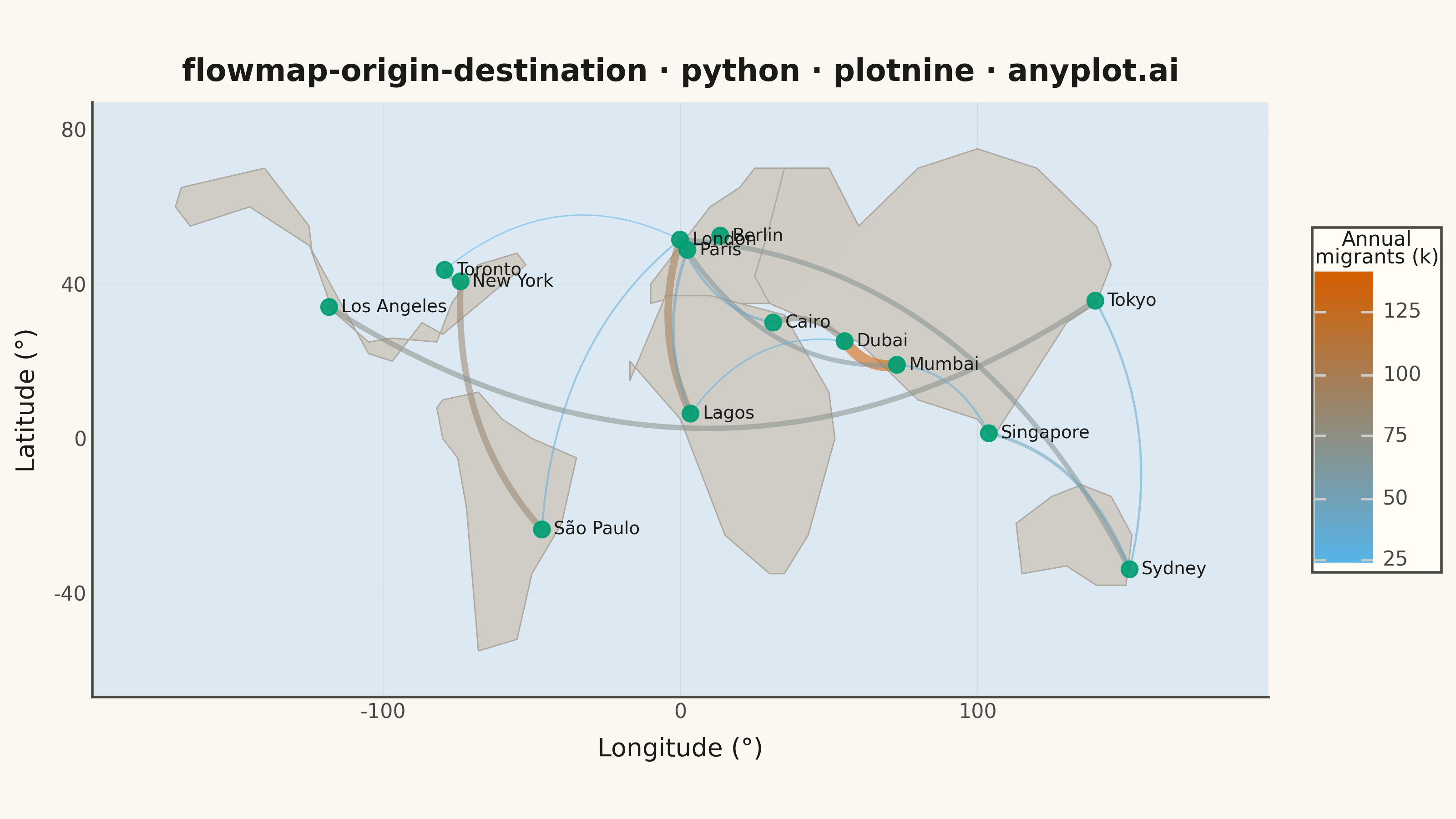
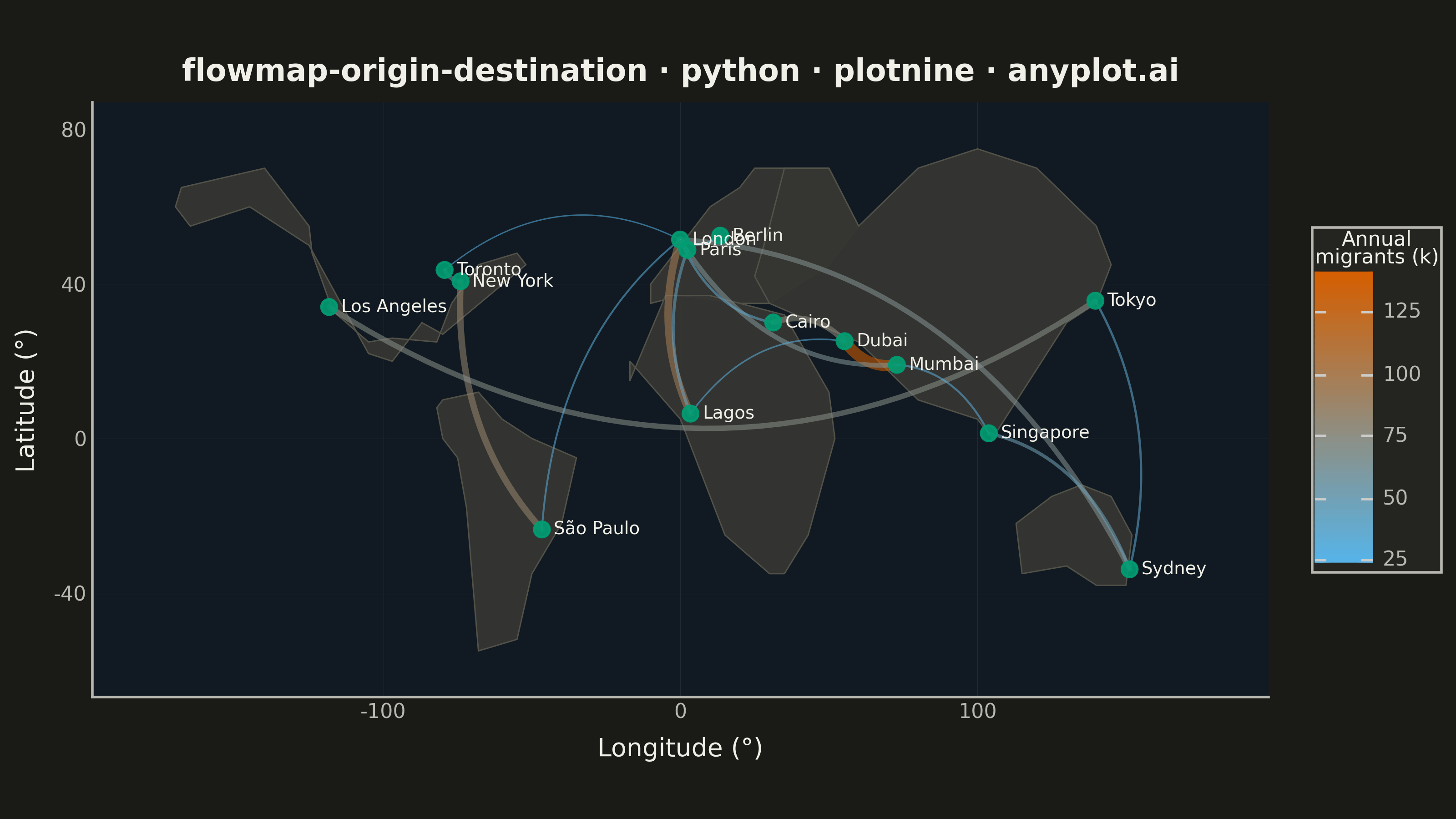
An origin-destination flow map visualizes movement or transfer between geographic locations using curved arcs overlaid on a map. Each arc connects an origin point to a destination point, with line thickness proportional to the flow magnitude. This visualization excels at revealing spatial patterns in migration, trade, or travel data, making it easy to identify major corridors, hub locations, and directional imbalances in movement between places.
""" anyplot.ai
flowmap-origin-destination: Origin-Destination Flow Map
Library: plotnine 0.15.4 | Python 3.13.13
Quality: 83/100 | Updated: 2026-05-20
"""

import os

import numpy as np
import pandas as pd
from plotnine import (
    aes,
    coord_fixed,
    element_blank,
    element_line,
    element_rect,
    element_text,
    geom_path,
    geom_point,
    geom_polygon,
    geom_text,
    ggplot,
    labs,
    scale_color_cmap,
    scale_size_identity,
    theme,
    theme_minimal,
)


THEME = os.getenv("ANYPLOT_THEME", "light")
PAGE_BG = "#FAF8F1" if THEME == "light" else "#1A1A17"
ELEVATED_BG = "#FFFDF6" if THEME == "light" else "#242420"
INK = "#1A1A17" if THEME == "light" else "#F0EFE8"
INK_SOFT = "#4A4A44" if THEME == "light" else "#B8B7B0"
OCEAN_BG = "#DDE9F2" if THEME == "light" else "#111A22"
LAND_FILL = "#D0CCC4" if THEME == "light" else "#363632"
LAND_COLOR = "#AEA9A1" if THEME == "light" else "#525248"

# Major world cities (lat, lon)
locations = {
    "New York": (40.71, -74.01),
    "London": (51.51, -0.13),
    "Paris": (48.85, 2.35),
    "Dubai": (25.20, 55.27),
    "Sydney": (-33.87, 151.21),
    "Toronto": (43.65, -79.38),
    "Singapore": (1.35, 103.82),
    "Tokyo": (35.68, 139.69),
    "São Paulo": (-23.55, -46.63),
    "Mumbai": (19.08, 72.88),
    "Lagos": (6.45, 3.40),
    "Cairo": (30.04, 31.24),
    "Berlin": (52.52, 13.40),
    "Los Angeles": (34.05, -118.24),
}

# International migration flows (thousands of people per year)
flows_data = [
    ("Mumbai", "Dubai", 142),
    ("Lagos", "London", 98),
    ("São Paulo", "New York", 85),
    ("Cairo", "Dubai", 78),
    ("Tokyo", "Los Angeles", 72),
    ("London", "Sydney", 68),
    ("Mumbai", "London", 65),
    ("New York", "Toronto", 60),
    ("Paris", "London", 55),
    ("Singapore", "Sydney", 48),
    ("Lagos", "Paris", 44),
    ("Berlin", "London", 40),
    ("Cairo", "London", 38),
    ("Tokyo", "Sydney", 35),
    ("Mumbai", "Singapore", 32),
    ("São Paulo", "London", 30),
    ("Lagos", "Dubai", 27),
    ("Toronto", "London", 24),
]

# Build flow path data with inline quadratic Bezier curve computation
flow_paths = []
flow_values = [f for _, _, f in flows_data]
min_flow = float(min(flow_values))
max_flow = float(max(flow_values))

for i, (origin, dest, flow) in enumerate(flows_data):
    origin_lat, origin_lon = locations[origin]
    dest_lat, dest_lon = locations[dest]

    mid_x = (origin_lon + dest_lon) / 2
    mid_y = (origin_lat + dest_lat) / 2
    dx = dest_lon - origin_lon
    dy = dest_lat - origin_lat
    seg_len = np.sqrt(dx**2 + dy**2)
    perp_x = -dy / seg_len if seg_len > 0 else 0.0
    perp_y = dx / seg_len if seg_len > 0 else 0.0
    ctrl_x = mid_x + perp_x * seg_len * 0.25
    ctrl_y = mid_y + perp_y * seg_len * 0.25

    line_width = 0.3 + ((flow - min_flow) / (max_flow - min_flow)) * 2.2
    t = np.linspace(0, 1, 40)
    curve_x = (1 - t) ** 2 * origin_lon + 2 * (1 - t) * t * ctrl_x + t**2 * dest_lon
    curve_y = (1 - t) ** 2 * origin_lat + 2 * (1 - t) * t * ctrl_y + t**2 * dest_lat

    for j in range(len(t)):
        flow_paths.append(
            {"flow_id": i, "order": j, "x": curve_x[j], "y": curve_y[j], "flow": float(flow), "size": line_width}
        )

df_flows = pd.DataFrame(flow_paths)

# Per-city label nudge (degrees) to separate the dense Western Europe cluster
LABEL_NUDGE = {
    "London": (4, 3.0),  # nudge up to clear Paris
    "Paris": (4, -3.0),  # nudge down to clear London/Berlin
    "Berlin": (4, 2.5),  # nudge up, east of Paris so less conflict
    "Toronto": (4, 2.0),  # nudge up (near New York)
    "New York": (4, -2.0),  # nudge down (near Toronto)
}
DEFAULT_NUDGE = (4, 0)

location_points = []
for name, (lat, lon) in locations.items():
    nx, ny = LABEL_NUDGE.get(name, DEFAULT_NUDGE)
    location_points.append({"name": name, "lat": lat, "lon": lon, "lx": lon + nx, "ly": lat + ny})
df_locations = pd.DataFrame(location_points)

# Simplified continent outlines for basemap
continents = []

# North America
na_lon = [
    -170,
    -168,
    -140,
    -125,
    -124,
    -117,
    -105,
    -97,
    -82,
    -77,
    -68,
    -55,
    -52,
    -80,
    -87,
    -97,
    -105,
    -125,
    -145,
    -165,
    -170,
]
na_lat = [60, 65, 70, 55, 48, 33, 25, 26, 25, 35, 45, 48, 45, 27, 30, 20, 22, 50, 60, 55, 60]
for i in range(len(na_lon)):
    continents.append({"continent": "N. America", "order": i, "lon": na_lon[i], "lat": na_lat[i]})

# South America
sa_lon = [-80, -68, -60, -50, -35, -40, -50, -55, -68, -72, -75, -80, -82, -80]
sa_lat = [10, 12, 5, 0, -5, -22, -35, -52, -55, -18, -5, 0, 8, 10]
for i in range(len(sa_lon)):
    continents.append({"continent": "S. America", "order": i, "lon": sa_lon[i], "lat": sa_lat[i]})

# Europe
eu_lon = [-10, 0, 10, 20, 30, 40, 50, 60, 50, 35, 25, 20, 10, 0, -10, -10]
eu_lat = [35, 37, 36, 35, 35, 40, 45, 55, 70, 70, 70, 65, 60, 50, 40, 35]
for i in range(len(eu_lon)):
    continents.append({"continent": "Europe", "order": i, "lon": eu_lon[i], "lat": eu_lat[i]})

# Africa
af_lon = [-17, -5, 10, 35, 50, 52, 43, 35, 30, 15, 0, -17, -17]
af_lat = [15, 37, 37, 32, 12, 0, -25, -35, -35, -25, 5, 20, 15]
for i in range(len(af_lon)):
    continents.append({"continent": "Africa", "order": i, "lon": af_lon[i], "lat": af_lat[i]})

# Asia
as_lon = [60, 80, 100, 120, 140, 145, 140, 130, 105, 100, 80, 60, 45, 30, 25, 30, 35, 50, 60]
as_lat = [55, 70, 75, 70, 55, 45, 35, 30, 0, 5, 10, 25, 30, 35, 42, 55, 70, 70, 55]
for i in range(len(as_lon)):
    continents.append({"continent": "Asia", "order": i, "lon": as_lon[i], "lat": as_lat[i]})

# Australia/Oceania
au_lon = [113, 125, 135, 145, 152, 150, 140, 130, 115, 113]
au_lat = [-22, -15, -12, -15, -25, -38, -38, -33, -35, -22]
for i in range(len(au_lon)):
    continents.append({"continent": "Australia", "order": i, "lon": au_lon[i], "lat": au_lat[i]})

df_continents = pd.DataFrame(continents)

# Build the origin-destination flow map
plot = (
    ggplot()
    + geom_polygon(
        aes(x="lon", y="lat", group="continent"),
        data=df_continents,
        fill=LAND_FILL,
        color=LAND_COLOR,
        size=0.3,
        alpha=0.7,
    )
    + geom_path(
        aes(x="x", y="y", group="flow_id", color="flow", size="size"), data=df_flows, alpha=0.55, lineend="round"
    )
    + geom_point(aes(x="lon", y="lat"), data=df_locations, color="#009E73", size=3.0, alpha=0.9)
    + geom_text(aes(x="lx", y="ly", label="name"), data=df_locations, color=INK, size=8, ha="left")
    + scale_size_identity()
    + scale_color_cmap(cmap_name="viridis", name="Annual\nmigrants (k)", limits=(min_flow, max_flow))
    + coord_fixed(ratio=1.3, xlim=(-180, 180), ylim=(-60, 80))
    + labs(title="flowmap-origin-destination · python · plotnine · anyplot.ai", x="Longitude (°)", y="Latitude (°)")
    + theme_minimal()
    + theme(
        figure_size=(8, 4.5),
        plot_background=element_rect(fill=PAGE_BG, color=PAGE_BG),
        panel_background=element_rect(fill=OCEAN_BG),
        panel_grid_major=element_line(color=INK, size=0.2, alpha=0.08),
        panel_grid_minor=element_blank(),
        axis_line=element_line(color=INK_SOFT),
        plot_title=element_text(size=12, color=INK, weight="bold"),
        axis_title=element_text(size=10, color=INK),
        axis_text=element_text(size=8, color=INK_SOFT),
        legend_title=element_text(size=8, color=INK),
        legend_text=element_text(size=8, color=INK_SOFT),
        legend_background=element_rect(fill=ELEVATED_BG, color=INK_SOFT),
        legend_position="right",
    )
)

plot.save(f"plot-{THEME}.png", dpi=400, width=8, height=4.5, units="in", verbose=False)
Runnable source as JSON, for any HTTP client: https://api.anyplot.ai/specs/flowmap-origin-destination/plotnine/code. Any spec id and library id listed in llms-full.txt fit the same URL shape; every URL below is complete and callable.
{
  "spec_id": "flowmap-origin-destination",
  "language": "python",
  "library": "plotnine",
  "page": "https://anyplot.ai/flowmap-origin-destination/python/plotnine",
  "hub": "https://anyplot.ai/flowmap-origin-destination",
  "code_json": "https://api.anyplot.ai/specs/flowmap-origin-destination/plotnine/code",
  "spec_json": "https://api.anyplot.ai/specs/flowmap-origin-destination",
  "render_light_png": "https://storage.googleapis.com/anyplot-images/plots/flowmap-origin-destination/python/plotnine/plot-light.png",
  "render_dark_png": "https://storage.googleapis.com/anyplot-images/plots/flowmap-origin-destination/python/plotnine/plot-dark.png",
  "quality_score": 83.0,
  "license": "MIT",
  "guide": "https://anyplot.ai/llms.txt"
}
Part of Origin-Destination Flow Map on anyplot.ai.