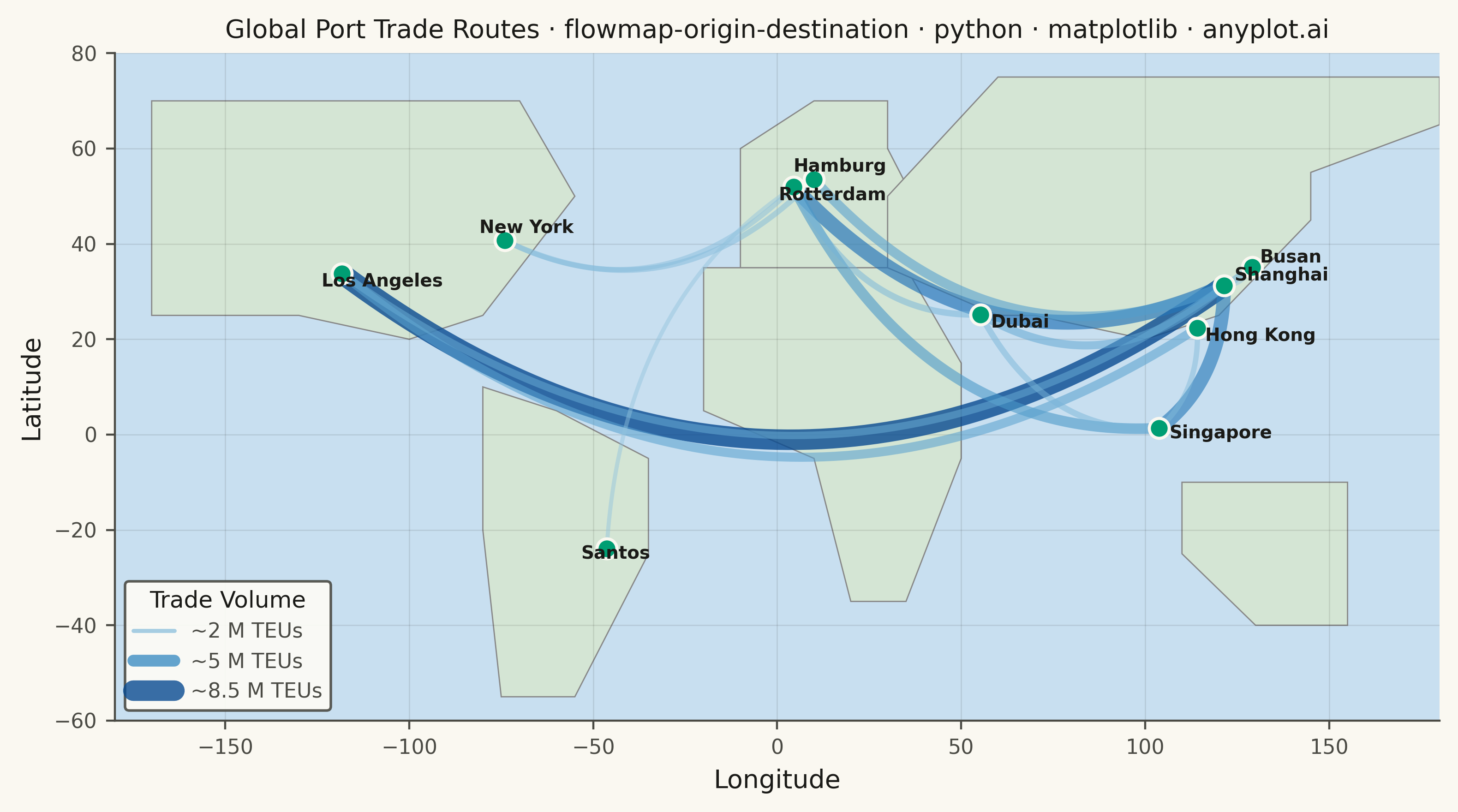
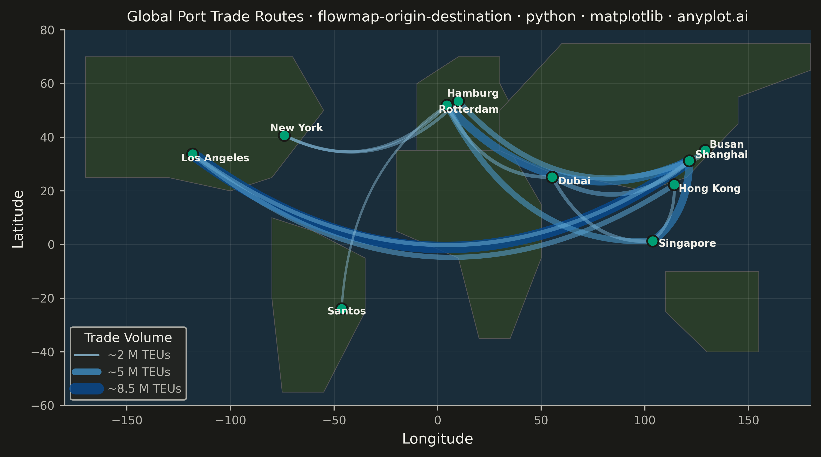
An origin-destination flow map visualizes movement or transfer between geographic locations using curved arcs overlaid on a map. Each arc connects an origin point to a destination point, with line thickness proportional to the flow magnitude. This visualization excels at revealing spatial patterns in migration, trade, or travel data, making it easy to identify major corridors, hub locations, and directional imbalances in movement between places.
""" anyplot.ai
flowmap-origin-destination: Origin-Destination Flow Map
Library: matplotlib 3.10.9 | Python 3.13.13
Quality: 83/100 | Updated: 2026-05-20
"""

import os

import matplotlib.lines as mlines
import matplotlib.pyplot as plt
import numpy as np


# Theme tokens
THEME = os.getenv("ANYPLOT_THEME", "light")
PAGE_BG = "#FAF8F1" if THEME == "light" else "#1A1A17"
ELEVATED_BG = "#FFFDF6" if THEME == "light" else "#242420"
INK = "#1A1A17" if THEME == "light" else "#F0EFE8"
INK_SOFT = "#4A4A44" if THEME == "light" else "#B8B7B0"
INK_MUTED = "#6B6A63" if THEME == "light" else "#A8A79F"
LAND_COLOR = "#D4E5D4" if THEME == "light" else "#2A3D2A"
OCEAN_COLOR = "#C8DFF0" if THEME == "light" else "#1A2D3A"
BORDER_COLOR = "#888888" if THEME == "light" else "#555555"

# Data - Trade flows between major world ports
np.random.seed(42)

# Major port cities with coordinates (lon, lat)
ports = {
    "Shanghai": (121.47, 31.23),
    "Singapore": (103.82, 1.35),
    "Rotterdam": (4.48, 51.92),
    "Los Angeles": (-118.25, 33.75),
    "Dubai": (55.27, 25.20),
    "Hong Kong": (114.17, 22.32),
    "Busan": (129.03, 35.10),
    "Hamburg": (9.99, 53.55),
    "New York": (-74.00, 40.71),
    "Santos": (-46.33, -23.95),
}

# Define trade flows (origin, destination, flow volume in million TEUs)
flows = [
    ("Shanghai", "Los Angeles", 8.5),
    ("Shanghai", "Rotterdam", 6.2),
    ("Shanghai", "Singapore", 5.8),
    ("Singapore", "Rotterdam", 4.5),
    ("Hong Kong", "Los Angeles", 3.9),
    ("Busan", "Los Angeles", 3.2),
    ("Dubai", "Rotterdam", 2.8),
    ("Hamburg", "New York", 2.5),
    ("Rotterdam", "New York", 2.3),
    ("Santos", "Rotterdam", 1.9),
    ("Shanghai", "Dubai", 3.5),
    ("Singapore", "Dubai", 2.7),
    ("Hong Kong", "Singapore", 2.4),
    ("Shanghai", "Hamburg", 4.1),
    ("Busan", "Shanghai", 1.8),
]

# Label offsets to avoid overlap (lon_offset, lat_offset)
label_offsets = {
    "Shanghai": (4, 2),
    "Singapore": (4, -4),
    "Rotterdam": (-6, -5),
    "Los Angeles": (-8, -5),
    "Dubai": (4, -5),
    "Hong Kong": (3, -5),
    "Busan": (3, 2),
    "Hamburg": (-8, 3),
    "New York": (-10, 3),
    "Santos": (-10, -4),
}

# Plot
fig, ax = plt.subplots(figsize=(8, 4.5), dpi=400, facecolor=PAGE_BG)
ax.set_facecolor(OCEAN_COLOR)
ax.set_xlim(-180, 180)
ax.set_ylim(-60, 80)

# Simplified continent outlines
continent_coords = [
    [
        (-170, 60),
        (-170, 25),
        (-130, 25),
        (-100, 20),
        (-80, 25),
        (-60, 45),
        (-55, 50),
        (-70, 70),
        (-170, 70),
        (-170, 60),
    ],
    [(-80, 10), (-60, 5), (-35, -5), (-35, -25), (-55, -55), (-75, -55), (-80, -20), (-80, 10)],
    [(-10, 35), (0, 35), (30, 35), (40, 45), (30, 60), (30, 70), (10, 70), (-10, 60), (-10, 35)],
    [(-20, 35), (35, 35), (50, 15), (50, -5), (35, -35), (20, -35), (10, -5), (-20, 5), (-20, 35)],
    [
        (30, 35),
        (60, 25),
        (70, 25),
        (100, 20),
        (120, 25),
        (145, 45),
        (145, 55),
        (180, 65),
        (180, 75),
        (60, 75),
        (30, 50),
        (30, 35),
    ],
    [(110, -10), (155, -10), (155, -40), (130, -40), (110, -25), (110, -10)],
]

for coords in continent_coords:
    xs = [c[0] for c in coords]
    ys = [c[1] for c in coords]
    ax.fill(xs, ys, color=LAND_COLOR, edgecolor=BORDER_COLOR, linewidth=0.5, zorder=1)

# Normalize flow values for line width scaling
max_flow = max(f[2] for f in flows)
min_flow = min(f[2] for f in flows)

# Draw flows using quadratic Bezier curves
t = np.linspace(0, 1, 80)
height_factor = 0.28

for origin_name, dest_name, flow in flows:
    ox, oy = ports[origin_name]
    dx, dy = ports[dest_name]

    mx, my = (ox + dx) / 2, (oy + dy) / 2
    distance = np.sqrt((dx - ox) ** 2 + (dy - oy) ** 2)

    if distance > 0:
        px, py = -(dy - oy) / distance, (dx - ox) / distance
    else:
        px, py = 0, 1

    cx = mx + px * distance * height_factor
    cy = my + py * distance * height_factor

    x = (1 - t) ** 2 * ox + 2 * (1 - t) * t * cx + t**2 * dx
    y = (1 - t) ** 2 * oy + 2 * (1 - t) * t * cy + t**2 * dy

    normalized = (flow - min_flow) / (max_flow - min_flow) if max_flow > min_flow else 0.5
    line_width = 1.5 + normalized * 6.5
    alpha = 0.45 + normalized * 0.35

    # Blue colormap works well in both light and dark themes
    color = plt.cm.Blues(0.4 + normalized * 0.5)
    ax.plot(x, y, color=color, linewidth=line_width, alpha=alpha, zorder=3, solid_capstyle="round")

# Draw port markers — brand green for single categorical series (Okabe-Ito position 1)
for port_name, (lon, lat) in ports.items():
    ax.scatter(lon, lat, s=60, c="#009E73", edgecolors=PAGE_BG, linewidths=1.2, zorder=4)
    lon_off, lat_off = label_offsets.get(port_name, (4, 3))
    ax.annotate(
        port_name,
        (lon, lat),
        xytext=(lon_off, lat_off),
        textcoords="offset points",
        fontsize=7,
        fontweight="bold",
        color=INK,
        zorder=5,
    )

# Legend with actual line samples to reflect line-width encoding
legend_levels = [(1.9, "~2 M TEUs"), (5.0, "~5 M TEUs"), (8.5, "~8.5 M TEUs")]
legend_handles = []
for lf, label in legend_levels:
    normalized = (lf - min_flow) / (max_flow - min_flow)
    lw = 1.5 + normalized * 6.5
    color = plt.cm.Blues(0.4 + normalized * 0.5)
    handle = mlines.Line2D([], [], color=color, linewidth=lw, label=label, alpha=0.8, solid_capstyle="round")
    legend_handles.append(handle)

leg = ax.legend(
    handles=legend_handles,
    loc="lower left",
    fontsize=8,
    title="Trade Volume",
    title_fontsize=9,
    framealpha=0.9,
    facecolor=ELEVATED_BG,
    edgecolor=INK_SOFT,
)
plt.setp(leg.get_title(), color=INK)
plt.setp(leg.get_texts(), color=INK_SOFT)

# Style
ax.set_xlabel("Longitude", fontsize=10, color=INK)
ax.set_ylabel("Latitude", fontsize=10, color=INK)
ax.set_title(
    "Global Port Trade Routes · flowmap-origin-destination · python · matplotlib · anyplot.ai",
    fontsize=10,
    fontweight="medium",
    color=INK,
)
ax.tick_params(axis="both", labelsize=8, colors=INK_SOFT)
for s in ("left", "bottom"):
    ax.spines[s].set_color(INK_SOFT)
ax.spines["top"].set_visible(False)
ax.spines["right"].set_visible(False)
ax.grid(True, alpha=0.10, linewidth=0.5, color=INK, zorder=0)

plt.tight_layout()
plt.savefig(f"plot-{THEME}.png", dpi=400, bbox_inches="tight", facecolor=PAGE_BG)
Runnable source as JSON, for any HTTP client: https://api.anyplot.ai/specs/flowmap-origin-destination/matplotlib/code. Any spec id and library id listed in llms-full.txt fit the same URL shape; every URL below is complete and callable.
{
  "spec_id": "flowmap-origin-destination",
  "language": "python",
  "library": "matplotlib",
  "page": "https://anyplot.ai/flowmap-origin-destination/python/matplotlib",
  "hub": "https://anyplot.ai/flowmap-origin-destination",
  "code_json": "https://api.anyplot.ai/specs/flowmap-origin-destination/matplotlib/code",
  "spec_json": "https://api.anyplot.ai/specs/flowmap-origin-destination",
  "render_light_png": "https://storage.googleapis.com/anyplot-images/plots/flowmap-origin-destination/python/matplotlib/plot-light.png",
  "render_dark_png": "https://storage.googleapis.com/anyplot-images/plots/flowmap-origin-destination/python/matplotlib/plot-dark.png",
  "quality_score": 83.0,
  "license": "MIT",
  "guide": "https://anyplot.ai/llms.txt"
}
Part of Origin-Destination Flow Map on anyplot.ai.