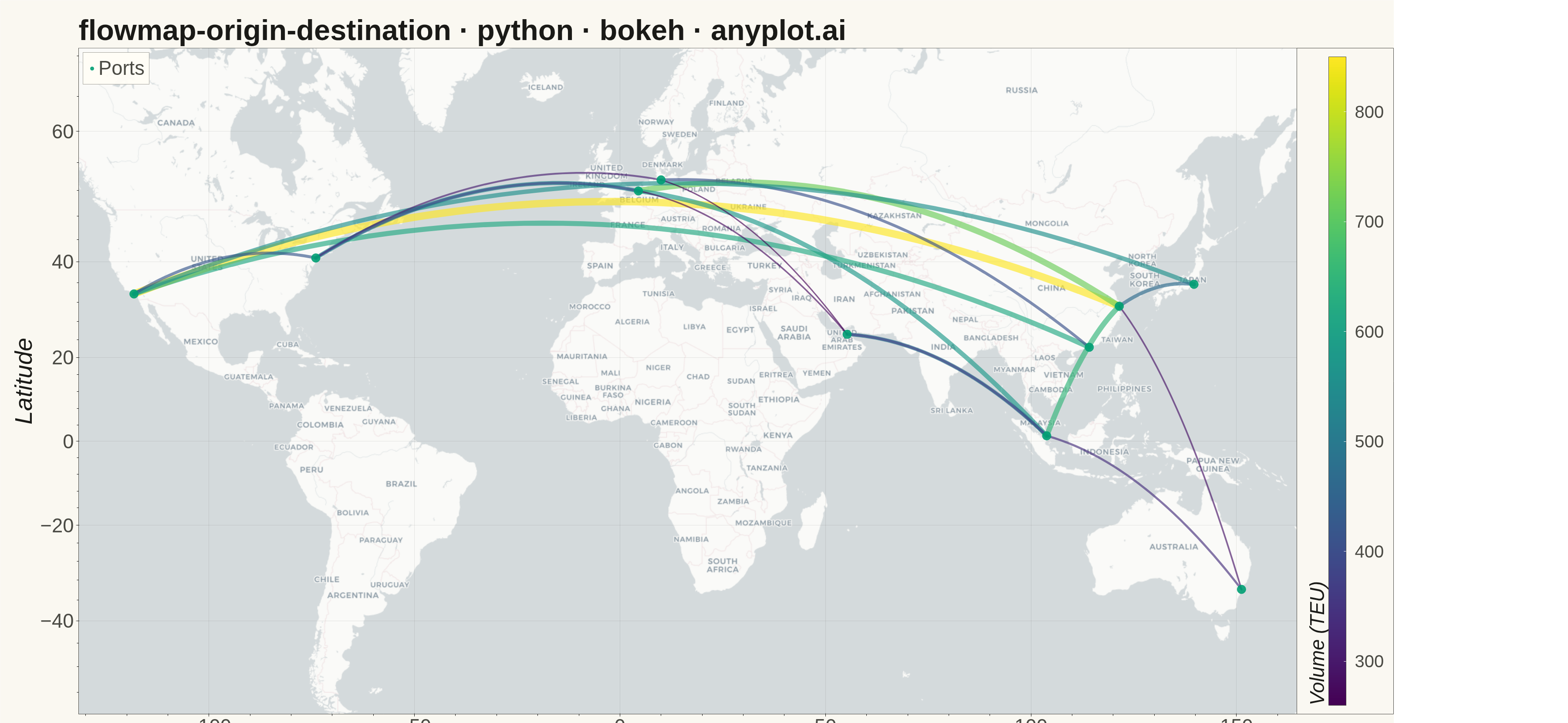
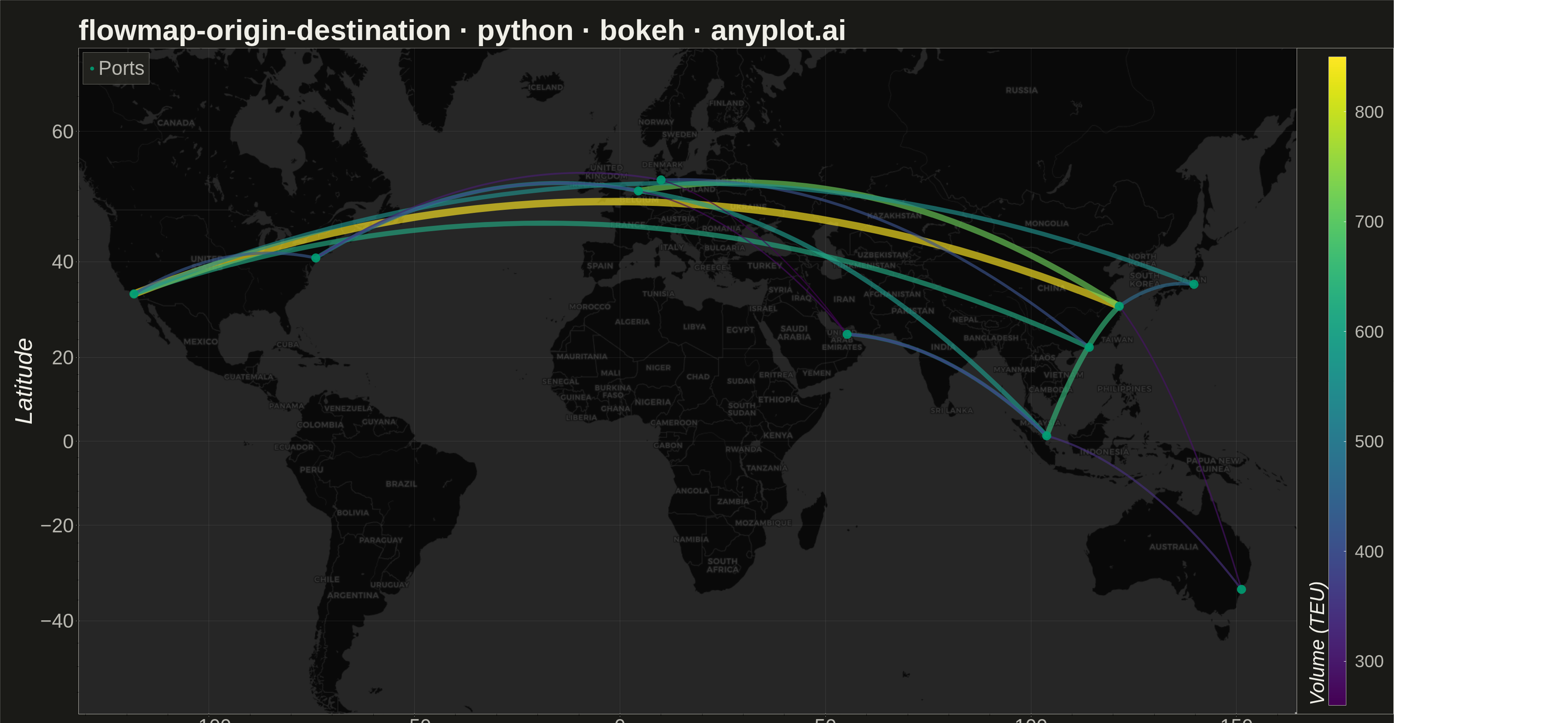
An origin-destination flow map visualizes movement or transfer between geographic locations using curved arcs overlaid on a map. Each arc connects an origin point to a destination point, with line thickness proportional to the flow magnitude. This visualization excels at revealing spatial patterns in migration, trade, or travel data, making it easy to identify major corridors, hub locations, and directional imbalances in movement between places.
""" anyplot.ai
flowmap-origin-destination: Origin-Destination Flow Map
Library: bokeh 3.9.0 | Python 3.13.13
Quality: 88/100 | Updated: 2026-05-20
"""

import os
import sys
import time
from pathlib import Path


# This file is named bokeh.py — remove its directory from sys.path so that
# `import bokeh` resolves to the installed package, not this file itself.
sys.path = [p for p in sys.path if Path(p).resolve() != Path(__file__).resolve().parent]

import numpy as np
import pandas as pd
from bokeh.io import output_file, save
from bokeh.models import ColorBar, ColumnDataSource, HoverTool, LinearColorMapper, WMTSTileSource
from bokeh.palettes import Viridis256
from bokeh.plotting import figure
from selenium import webdriver
from selenium.webdriver.chrome.options import Options


# Theme tokens
THEME = os.getenv("ANYPLOT_THEME", "light")
PAGE_BG = "#FAF8F1" if THEME == "light" else "#1A1A17"
ELEVATED_BG = "#FFFDF6" if THEME == "light" else "#242420"
INK = "#1A1A17" if THEME == "light" else "#F0EFE8"
INK_SOFT = "#4A4A44" if THEME == "light" else "#B8B7B0"

# Data: Global maritime trade flows between major ports
np.random.seed(42)

ports = {
    "Shanghai": (31.2304, 121.4737),
    "Singapore": (1.3521, 103.8198),
    "Rotterdam": (51.9225, 4.4792),
    "Los Angeles": (33.7490, -118.2437),
    "Dubai": (25.2048, 55.2708),
    "Hong Kong": (22.3193, 114.1694),
    "Hamburg": (53.5511, 9.9937),
    "New York": (40.7128, -74.0060),
    "Tokyo": (35.6762, 139.6503),
    "Sydney": (-33.8688, 151.2093),
}

flow_pairs = [
    ("Shanghai", "Los Angeles", 850),
    ("Shanghai", "Rotterdam", 720),
    ("Singapore", "Rotterdam", 580),
    ("Singapore", "Dubai", 490),
    ("Hong Kong", "Los Angeles", 620),
    ("Hong Kong", "Hamburg", 410),
    ("Rotterdam", "New York", 530),
    ("Dubai", "Singapore", 380),
    ("Tokyo", "Los Angeles", 560),
    ("Tokyo", "Shanghai", 470),
    ("Shanghai", "Singapore", 650),
    ("Los Angeles", "New York", 420),
    ("Sydney", "Singapore", 340),
    ("Sydney", "Shanghai", 290),
    ("Hamburg", "New York", 310),
    ("Rotterdam", "Dubai", 280),
    ("New York", "Rotterdam", 390),
    ("Dubai", "Hamburg", 260),
]

df = pd.DataFrame(
    [
        {
            "origin_name": origin,
            "dest_name": dest,
            "origin_lat": ports[origin][0],
            "origin_lon": ports[origin][1],
            "dest_lat": ports[dest][0],
            "dest_lon": ports[dest][1],
            "flow": flow,
        }
        for origin, dest, flow in flow_pairs
    ]
)

# Web Mercator projection (EPSG:3857) — inlined, no helper function
k = 6378137
df["origin_x"] = df["origin_lon"] * (k * np.pi / 180.0)
df["origin_y"] = np.log(np.tan((90 + df["origin_lat"]) * np.pi / 360.0)) * k
df["dest_x"] = df["dest_lon"] * (k * np.pi / 180.0)
df["dest_y"] = np.log(np.tan((90 + df["dest_lat"]) * np.pi / 360.0)) * k

# Flow encoding: proportional line width + viridis color (continuous data)
min_flow = df["flow"].min()
max_flow = df["flow"].max()
df["line_width"] = 3 + (df["flow"] - min_flow) / (max_flow - min_flow) * 14
color_mapper = LinearColorMapper(palette=Viridis256, low=min_flow, high=max_flow)
color_idx = ((df["flow"] - min_flow) / (max_flow - min_flow) * 255).astype(int).clip(0, 255)
df["line_color"] = [Viridis256[i] for i in color_idx]

# Quadratic Bezier arcs — inlined loop, no helper function
t = np.linspace(0, 1, 50)
arc_xs, arc_ys = [], []
for _, row in df.iterrows():
    x0, y0 = row["origin_x"], row["origin_y"]
    x1, y1 = row["dest_x"], row["dest_y"]
    mid_x = (x0 + x1) / 2
    mid_y = (y0 + y1) / 2
    dist = np.sqrt((x1 - x0) ** 2 + (y1 - y0) ** 2)
    ctrl_y = mid_y + dist * 0.2
    arc_xs.append(((1 - t) ** 2 * x0 + 2 * (1 - t) * t * mid_x + t**2 * x1).tolist())
    arc_ys.append(((1 - t) ** 2 * y0 + 2 * (1 - t) * t * ctrl_y + t**2 * y1).tolist())

arc_source = ColumnDataSource(
    {
        "xs": arc_xs,
        "ys": arc_ys,
        "origin": df["origin_name"].tolist(),
        "dest": df["dest_name"].tolist(),
        "flow": df["flow"].tolist(),
        "line_width": df["line_width"].tolist(),
        "line_color": df["line_color"].tolist(),
    }
)

# Port marker data — inline mercator conversion
port_names = list(ports.keys())
port_lats = np.array([ports[n][0] for n in port_names])
port_lons = np.array([ports[n][1] for n in port_names])
port_source = ColumnDataSource(
    {
        "x": port_lons * (k * np.pi / 180.0),
        "y": np.log(np.tan((90 + port_lats) * np.pi / 360.0)) * k,
        "name": port_names,
        "lat": port_lats,
        "lon": port_lons,
    }
)

# Theme-adaptive basemap tile URL (WMTSTileSource — not deprecated string API)
tile_url = (
    "https://a.basemaps.cartocdn.com/light_all/{Z}/{X}/{Y}.png"
    if THEME == "light"
    else "https://a.basemaps.cartocdn.com/dark_all/{Z}/{X}/{Y}.png"
)

# Plot
p = figure(
    width=3200,
    height=1800,
    title="flowmap-origin-destination · python · bokeh · anyplot.ai",
    x_axis_type="mercator",
    y_axis_type="mercator",
    toolbar_location=None,
    min_border_bottom=160,
    min_border_left=180,
    min_border_top=110,
    min_border_right=50,
)

p.add_tile(WMTSTileSource(url=tile_url))

# Flow arcs via multi_line — single renderer enables per-arc hover tooltips
arcs = p.multi_line(
    xs="xs",
    ys="ys",
    source=arc_source,
    line_width="line_width",
    line_color="line_color",
    line_alpha=0.65,
    line_cap="round",
)

# Port markers (Okabe-Ito position 1 — brand green)
ports_r = p.scatter(x="x", y="y", source=port_source, size=20, color="#009E73", alpha=0.9, legend_label="Ports")

# Hover tools — arcs and port markers both interactive
p.add_tools(
    HoverTool(renderers=[arcs], tooltips=[("Route", "@origin → @dest"), ("Volume", "@flow{,} TEU")]),
    HoverTool(renderers=[ports_r], tooltips=[("Port", "@name"), ("Lat", "@lat{0.00}°"), ("Lon", "@lon{0.00}°")]),
)

# Chrome — theme-adaptive colors
p.background_fill_color = PAGE_BG
p.border_fill_color = PAGE_BG
p.outline_line_color = INK_SOFT

p.title.text_font_size = "50pt"
p.title.text_color = INK

p.xaxis.axis_label = "Longitude"
p.yaxis.axis_label = "Latitude"
p.xaxis.axis_label_text_font_size = "42pt"
p.yaxis.axis_label_text_font_size = "42pt"
p.xaxis.major_label_text_font_size = "34pt"
p.yaxis.major_label_text_font_size = "34pt"
p.xaxis.axis_label_text_color = INK
p.yaxis.axis_label_text_color = INK
p.xaxis.major_label_text_color = INK_SOFT
p.yaxis.major_label_text_color = INK_SOFT
p.xaxis.axis_line_color = INK_SOFT
p.yaxis.axis_line_color = INK_SOFT
p.xaxis.major_tick_line_color = INK_SOFT
p.yaxis.major_tick_line_color = INK_SOFT

p.xgrid.grid_line_color = INK
p.ygrid.grid_line_color = INK
p.xgrid.grid_line_alpha = 0.10
p.ygrid.grid_line_alpha = 0.10

p.legend.location = "top_left"
p.legend.label_text_font_size = "34pt"
p.legend.background_fill_color = ELEVATED_BG
p.legend.border_line_color = INK_SOFT
p.legend.label_text_color = INK_SOFT

# ColorBar — lets viewers quantify arc colors in TEU
color_bar = ColorBar(
    color_mapper=color_mapper,
    title="Volume (TEU)",
    title_text_font_size="34pt",
    title_text_color=INK,
    major_label_text_font_size="30pt",
    major_label_text_color=INK_SOFT,
    label_standoff=20,
    width=40,
    padding=20,
    background_fill_color=PAGE_BG,
    bar_line_color=INK_SOFT,
    border_line_color=INK_SOFT,
)
p.add_layout(color_bar, "right")

# Save HTML
output_file(f"plot-{THEME}.html")
save(p)

# Screenshot with headless Selenium (export_png uses snap chromedriver — broken)
# W is wider than figure width=3200 to accommodate the ColorBar right panel
W, H = 3600, 1800
opts = Options()
for arg in (
    "--headless=new",
    "--no-sandbox",
    "--disable-dev-shm-usage",
    "--disable-gpu",
    f"--window-size={W},{H}",
    "--hide-scrollbars",
):
    opts.add_argument(arg)
driver = webdriver.Chrome(options=opts)
driver.set_window_size(W, H)
driver.get(f"file://{Path(f'plot-{THEME}.html').resolve()}")
time.sleep(3)
driver.save_screenshot(f"plot-{THEME}.png")
driver.quit()
Runnable source as JSON, for any HTTP client: https://api.anyplot.ai/specs/flowmap-origin-destination/bokeh/code. Any spec id and library id listed in llms-full.txt fit the same URL shape; every URL below is complete and callable.
{
  "spec_id": "flowmap-origin-destination",
  "language": "python",
  "library": "bokeh",
  "page": "https://anyplot.ai/flowmap-origin-destination/python/bokeh",
  "hub": "https://anyplot.ai/flowmap-origin-destination",
  "code_json": "https://api.anyplot.ai/specs/flowmap-origin-destination/bokeh/code",
  "spec_json": "https://api.anyplot.ai/specs/flowmap-origin-destination",
  "render_light_png": "https://storage.googleapis.com/anyplot-images/plots/flowmap-origin-destination/python/bokeh/plot-light.png",
  "render_dark_png": "https://storage.googleapis.com/anyplot-images/plots/flowmap-origin-destination/python/bokeh/plot-dark.png",
  "interactive_light_html": "https://storage.googleapis.com/anyplot-images/plots/flowmap-origin-destination/python/bokeh/plot-light.html",
  "interactive_dark_html": "https://storage.googleapis.com/anyplot-images/plots/flowmap-origin-destination/python/bokeh/plot-dark.html",
  "quality_score": 88.0,
  "license": "MIT",
  "guide": "https://anyplot.ai/llms.txt"
}
Part of Origin-Destination Flow Map on anyplot.ai.