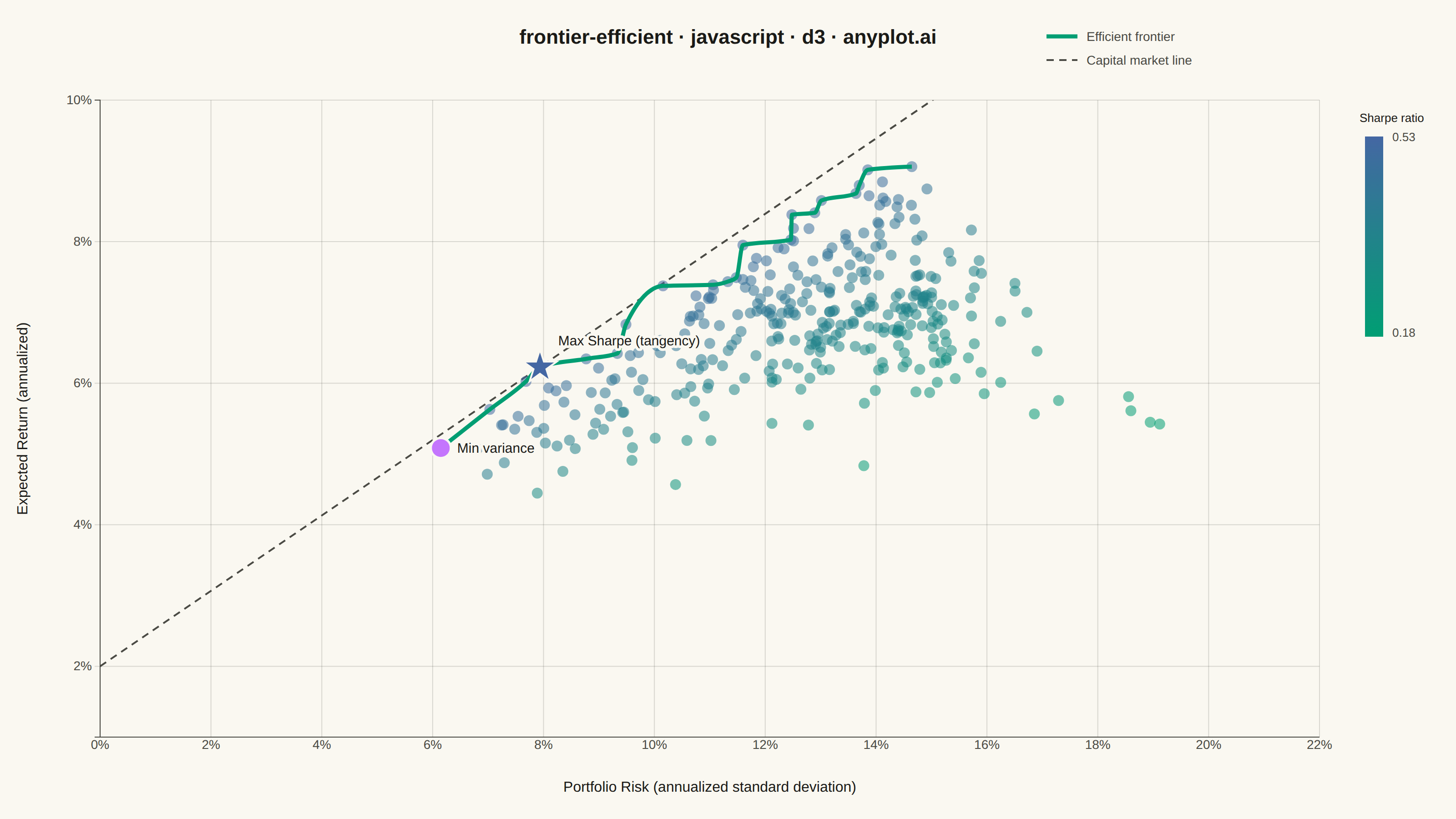
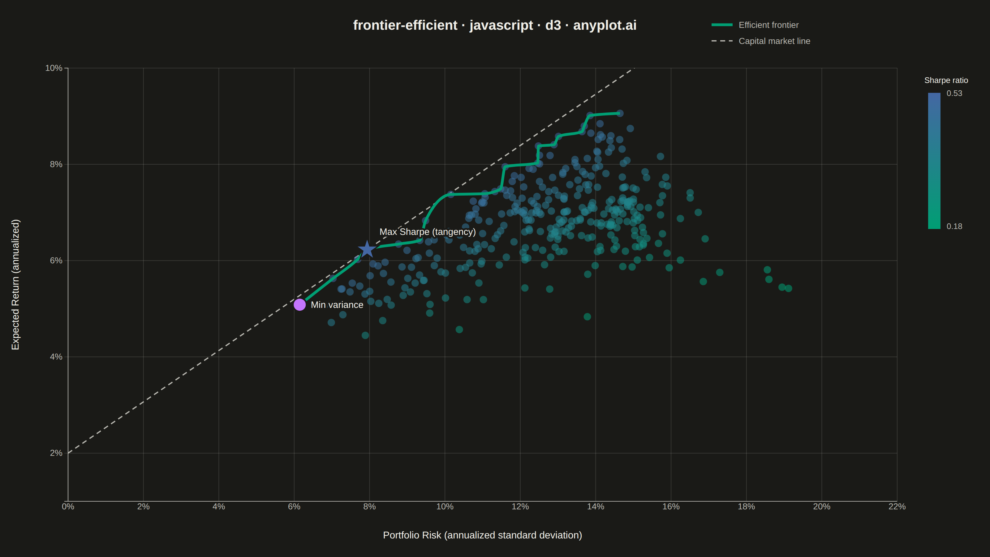
The same plot in 14 other libraries — JavaScript: Chart.js, Apache ECharts, Highcharts, MUI X Charts; Python: Altair, Bokeh, lets-plot, Matplotlib, Plotly, plotnine, Pygal, Seaborn; R: ggplot2; Julia: Makie.jl. Compare all 15 side by side: Efficient Frontier for Portfolio Optimization in Python, R, Julia and JavaScript.
The efficient frontier is a fundamental visualization in Modern Portfolio Theory (MPT) that displays a curve of optimal portfolios offering the highest expected return for each level of risk (standard deviation). Portfolios on the frontier are "efficient" because no other portfolio exists with higher return for the same risk, or lower risk for the same return. This plot is essential for asset allocation decisions and understanding the risk-return tradeoff in investment portfolios.
// anyplot.ai
// frontier-efficient: Efficient Frontier for Portfolio Optimization
// Library: d3 7.9.0 | JavaScript 22.23.2
// Quality: 89/100 | Created: 2026-09-02

const t = window.ANYPLOT_TOKENS;
const { width, height } = window.ANYPLOT_SIZE;
const margin = { top: 110, right: 150, bottom: 90, left: 110 };
const iw = width - margin.left - margin.right;
const ih = height - margin.top - margin.bottom;

// --- Data: Monte Carlo portfolio simulation over a 5-asset universe --------
function lcg(seed) {
  let state = seed;
  return function () {
    state = (state * 1103515245 + 12345) % 2147483648;
    return state / 2147483648;
  };
}
const rand = lcg(42);

const assets = [
  { name: "Bonds", return: 0.035, vol: 0.06 },
  { name: "REIT", return: 0.07, vol: 0.18 },
  { name: "Intl Equity", return: 0.08, vol: 0.19 },
  { name: "US Equity", return: 0.1, vol: 0.16 },
  { name: "Commodities", return: 0.05, vol: 0.22 },
];
const RISK_FREE = 0.02;

// One-factor market model: corr_ij = loading_i * loading_j (i != j). This
// guarantees a valid positive-semidefinite correlation matrix without having
// to hand-verify eigenvalues on a hand-picked 5x5 table.
const marketLoading = [0.05, 0.65, 0.75, 0.85, 0.55];
function correlation(i, j) {
  return i === j ? 1 : marketLoading[i] * marketLoading[j];
}
function covariance(i, j) {
  return correlation(i, j) * assets[i].vol * assets[j].vol;
}

function randomWeights(n) {
  const raw = Array.from({ length: n }, () => -Math.log(1 - rand()));
  const sum = raw.reduce((a, b) => a + b, 0);
  return raw.map((v) => v / sum);
}

const N_PORTFOLIOS = 350;
const portfolios = Array.from({ length: N_PORTFOLIOS }, () => {
  const w = randomWeights(assets.length);
  let ret = 0;
  for (let i = 0; i < assets.length; i++) ret += w[i] * assets[i].return;
  let variance = 0;
  for (let i = 0; i < assets.length; i++) {
    for (let j = 0; j < assets.length; j++) variance += w[i] * w[j] * covariance(i, j);
  }
  const risk = Math.sqrt(variance);
  return { risk, ret, sharpe: (ret - RISK_FREE) / risk };
});

// Efficient frontier: Pareto upper-left boundary of the simulated cloud —
// sort by risk, keep only portfolios that beat every lower-risk portfolio's
// return so far.
const byRisk = [...portfolios].sort((a, b) => a.risk - b.risk);
const frontier = [];
let bestRetSoFar = -Infinity;
for (const p of byRisk) {
  if (p.ret > bestRetSoFar) {
    frontier.push(p);
    bestRetSoFar = p.ret;
  }
}
const minVariance = frontier[0];
const maxSharpe = frontier.reduce((best, p) => (p.sharpe > best.sharpe ? p : best));

const maxRisk = d3.max(portfolios, (d) => d.risk);
const cmlEnd = { risk: maxRisk * 1.05, ret: RISK_FREE + maxSharpe.sharpe * maxRisk * 1.05 };

// --- Scales -------------------------------------------------------------
const x = d3
  .scaleLinear()
  .domain([0, maxRisk * 1.08])
  .nice()
  .range([0, iw]);
const y = d3
  .scaleLinear()
  .domain([RISK_FREE * 0.5, d3.max(portfolios, (d) => d.ret) * 1.08])
  .nice()
  .range([ih, 0]);
const sharpeExtent = d3.extent(portfolios, (d) => d.sharpe);
const color = d3.scaleSequential(d3.interpolateRgbBasis(t.seq)).domain(sharpeExtent);

// --- SVG mount ------------------------------------------------------------
const svg = d3.select("#container").append("svg").attr("width", width).attr("height", height);
const g = svg.append("g").attr("transform", `translate(${margin.left},${margin.top})`);
svg
  .append("clipPath")
  .attr("id", "plot-area-clip")
  .append("rect")
  .attr("width", iw)
  .attr("height", ih);

// --- Axes -------------------------------------------------------------
const pctFormat = d3.format(".0%");
const xAxis = g
  .append("g")
  .attr("transform", `translate(0,${ih})`)
  .call(d3.axisBottom(x).ticks(8).tickFormat(pctFormat).tickSize(-ih * 0.0));
const yAxis = g.append("g").call(d3.axisLeft(y).ticks(6).tickFormat(pctFormat));
for (const ax of [xAxis, yAxis]) {
  ax.selectAll("text").attr("fill", t.inkSoft).style("font-size", "14px");
  ax.selectAll("line").attr("stroke", t.grid);
  ax.select(".domain").attr("stroke", t.inkSoft);
}

// gridlines (both axes, subtle — this chart mixes scatter points with line series)
g.append("g")
  .attr("class", "grid")
  .call(d3.axisLeft(y).ticks(6).tickSize(-iw).tickFormat(""))
  .selectAll("line")
  .attr("stroke", t.grid);
g.select(".grid .domain").remove();

g.append("g")
  .attr("class", "grid")
  .attr("transform", `translate(0,${ih})`)
  .call(d3.axisBottom(x).ticks(8).tickSize(-ih).tickFormat(""))
  .selectAll("line")
  .attr("stroke", t.grid);
g.selectAll(".grid .domain").remove();

g.append("text")
  .attr("x", iw / 2)
  .attr("y", ih + 60)
  .attr("text-anchor", "middle")
  .attr("fill", t.ink)
  .style("font-size", "16px")
  .text("Portfolio Risk (annualized standard deviation)");
g.append("text")
  .attr("transform", "rotate(-90)")
  .attr("x", -ih / 2)
  .attr("y", -80)
  .attr("text-anchor", "middle")
  .attr("fill", t.ink)
  .style("font-size", "16px")
  .text("Expected Return (annualized)");

// --- Capital market line (risk-free tangent through the max-Sharpe portfolio)
const cmlLine = d3
  .line()
  .x((d) => x(d.risk))
  .y((d) => y(d.ret));
g.append("path")
  .datum([{ risk: 0, ret: RISK_FREE }, cmlEnd])
  .attr("clip-path", "url(#plot-area-clip)")
  .attr("fill", "none")
  .attr("stroke", t.inkSoft)
  .attr("stroke-width", 2)
  .attr("stroke-dasharray", "8,6")
  .attr("d", cmlLine);

// --- Random portfolio cloud, colored by Sharpe ratio -----------------------
g.selectAll("circle.portfolio")
  .data(portfolios)
  .join("circle")
  .attr("class", "portfolio")
  .attr("cx", (d) => x(d.risk))
  .attr("cy", (d) => y(d.ret))
  .attr("r", 6)
  .attr("fill", (d) => color(d.sharpe))
  .attr("fill-opacity", 0.55)
  .attr("stroke", "none");

// --- Efficient frontier curve (hero series — always brand green) ----------
const frontierLine = d3
  .line()
  .x((d) => x(d.risk))
  .y((d) => y(d.ret))
  .curve(d3.curveMonotoneX);
g.append("path")
  .datum(frontier)
  .attr("fill", "none")
  .attr("stroke", t.palette[0])
  .attr("stroke-width", 4.5)
  .attr("d", frontierLine);

// --- Key portfolios: minimum variance + maximum Sharpe (tangency) ---------
g.append("circle")
  .attr("cx", x(minVariance.risk))
  .attr("cy", y(minVariance.ret))
  .attr("r", 11)
  .attr("fill", t.palette[1])
  .attr("stroke", t.pageBg)
  .attr("stroke-width", 2.5);
g.append("text")
  .attr("x", x(minVariance.risk) + 18)
  .attr("y", y(minVariance.ret) + 5)
  .attr("fill", t.ink)
  .attr("stroke", t.pageBg)
  .attr("stroke-width", 6)
  .attr("stroke-linejoin", "round")
  .attr("paint-order", "stroke")
  .style("font-size", "15px")
  .text("Min variance");

g.append("path")
  .attr(
    "d",
    d3.symbol().type(d3.symbolStar).size(420)()
  )
  .attr("transform", `translate(${x(maxSharpe.risk)},${y(maxSharpe.ret)})`)
  .attr("fill", t.palette[2])
  .attr("stroke", t.pageBg)
  .attr("stroke-width", 2);
g.append("text")
  .attr("x", x(maxSharpe.risk) + 20)
  .attr("y", y(maxSharpe.ret) - 24)
  .attr("fill", t.ink)
  .attr("stroke", t.pageBg)
  .attr("stroke-width", 6)
  .attr("stroke-linejoin", "round")
  .attr("paint-order", "stroke")
  .style("font-size", "15px")
  .text("Max Sharpe (tangency)");

// --- Legend: frontier / CML swatches ---------------------------------------
const legend = g.append("g").attr("transform", `translate(${iw - 300}, -70)`);
const legendRows = [
  { label: "Efficient frontier", stroke: t.palette[0], dash: null, width: 4.5 },
  { label: "Capital market line", stroke: t.inkSoft, dash: "8,6", width: 2 },
];
legendRows.forEach((row, i) => {
  legend
    .append("line")
    .attr("x1", 0)
    .attr("x2", 34)
    .attr("y1", i * 26)
    .attr("y2", i * 26)
    .attr("stroke", row.stroke)
    .attr("stroke-width", row.width)
    .attr("stroke-dasharray", row.dash);
  legend
    .append("text")
    .attr("x", 44)
    .attr("y", i * 26 + 5)
    .attr("fill", t.inkSoft)
    .style("font-size", "14px")
    .text(row.label);
});

// --- Sharpe ratio color legend (vertical gradient bar) ----------------------
const legendGrad = svg
  .append("defs")
  .append("linearGradient")
  .attr("id", "sharpe-gradient")
  .attr("x1", "0%")
  .attr("y1", "100%")
  .attr("x2", "0%")
  .attr("y2", "0%");
d3.range(0, 1.001, 0.1).forEach((stop) => {
  legendGrad
    .append("stop")
    .attr("offset", `${stop * 100}%`)
    .attr("stop-color", color(sharpeExtent[0] + stop * (sharpeExtent[1] - sharpeExtent[0])));
});
const barX = margin.left + iw + 50;
const barY = margin.top + 40;
const barH = 220;
svg
  .append("rect")
  .attr("x", barX)
  .attr("y", barY)
  .attr("width", 20)
  .attr("height", barH)
  .attr("fill", "url(#sharpe-gradient)");
svg
  .append("text")
  .attr("x", barX + 30)
  .attr("y", barY + 5)
  .attr("fill", t.inkSoft)
  .style("font-size", "13px")
  .text(sharpeExtent[1].toFixed(2));
svg
  .append("text")
  .attr("x", barX + 30)
  .attr("y", barY + barH)
  .attr("fill", t.inkSoft)
  .style("font-size", "13px")
  .text(sharpeExtent[0].toFixed(2));
svg
  .append("text")
  .attr("x", barX - 6)
  .attr("y", barY - 16)
  .attr("fill", t.ink)
  .style("font-size", "13px")
  .text("Sharpe ratio");

// --- Title ------------------------------------------------------------
svg
  .append("text")
  .attr("x", width / 2)
  .attr("y", 48)
  .attr("text-anchor", "middle")
  .attr("fill", t.ink)
  .style("font-size", "22px")
  .style("font-weight", "600")
  .text("frontier-efficient · javascript · d3 · anyplot.ai");
Runnable source as JSON, for any HTTP client: https://api.anyplot.ai/specs/frontier-efficient/d3/code. Any spec id and library id listed in llms-full.txt fit the same URL shape; every URL below is complete and callable.
{
  "spec_id": "frontier-efficient",
  "language": "javascript",
  "library": "d3",
  "page": "https://anyplot.ai/frontier-efficient/javascript/d3",
  "hub": "https://anyplot.ai/frontier-efficient",
  "code_json": "https://api.anyplot.ai/specs/frontier-efficient/d3/code",
  "spec_json": "https://api.anyplot.ai/specs/frontier-efficient",
  "render_light_png": "https://storage.googleapis.com/anyplot-images/plots/frontier-efficient/javascript/d3/plot-light.png",
  "render_dark_png": "https://storage.googleapis.com/anyplot-images/plots/frontier-efficient/javascript/d3/plot-dark.png",
  "interactive_light_html": "https://storage.googleapis.com/anyplot-images/plots/frontier-efficient/javascript/d3/plot-light.html",
  "interactive_dark_html": "https://storage.googleapis.com/anyplot-images/plots/frontier-efficient/javascript/d3/plot-dark.html",
  "quality_score": 89.0,
  "license": "MIT",
  "guide": "https://anyplot.ai/llms.txt"
}
Part of Efficient Frontier for Portfolio Optimization on anyplot.ai.