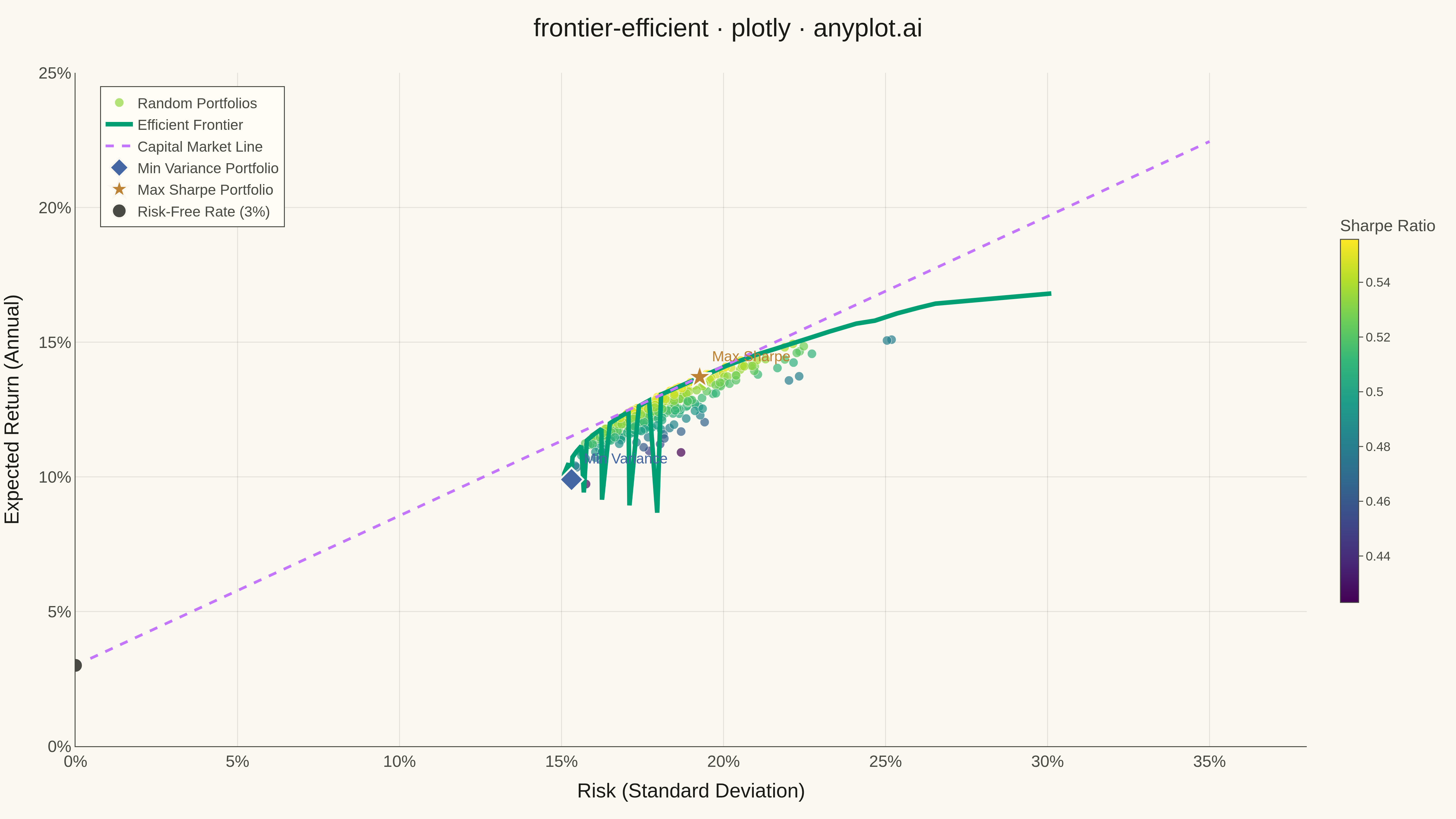
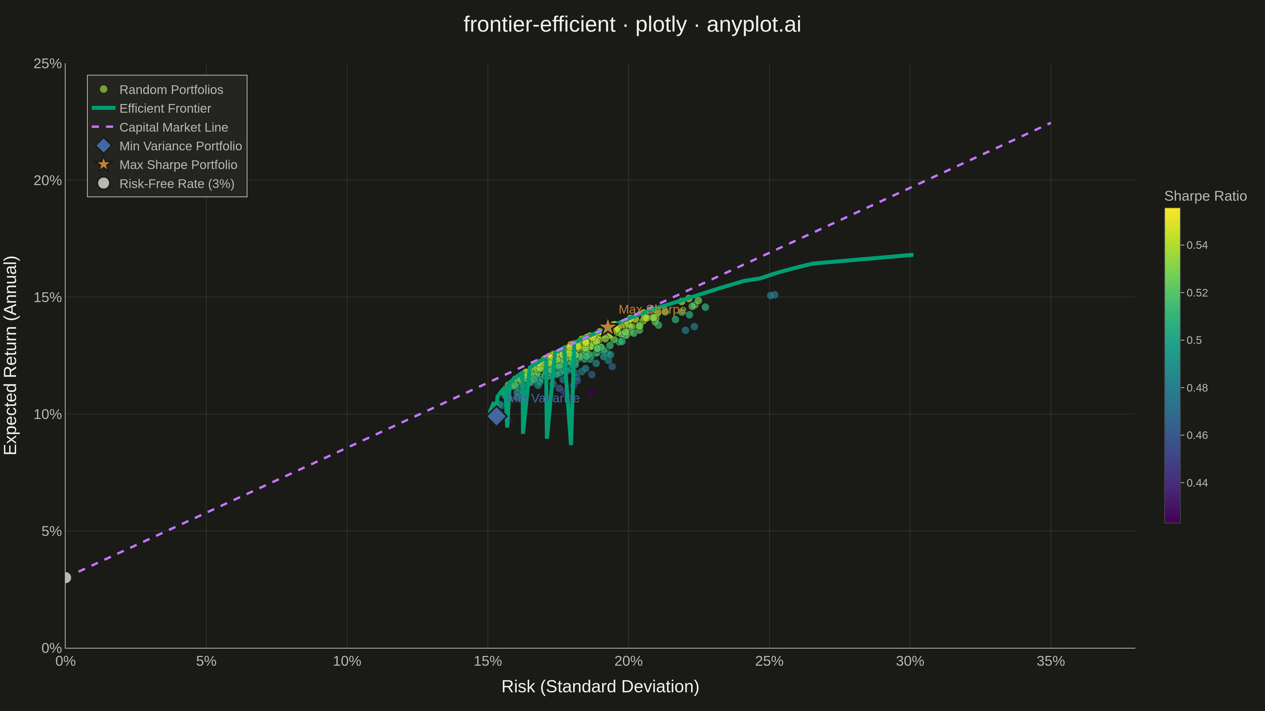
The efficient frontier is a fundamental visualization in Modern Portfolio Theory (MPT) that displays a curve of optimal portfolios offering the highest expected return for each level of risk (standard deviation). Portfolios on the frontier are "efficient" because no other portfolio exists with higher return for the same risk, or lower risk for the same return. This plot is essential for asset allocation decisions and understanding the risk-return tradeoff in investment portfolios.
""" anyplot.ai
frontier-efficient: Efficient Frontier for Portfolio Optimization
Library: plotly 6.7.0 | Python 3.13.13
Quality: 91/100 | Updated: 2026-05-17
"""

import os
import sys


# Remove current directory from path to avoid import collision with script filename
sys.path = [p for p in sys.path if p not in ("", ".", os.getcwd())]

import numpy as np
import plotly.graph_objects as go


# Theme tokens
THEME = os.getenv("ANYPLOT_THEME", "light")
PAGE_BG = "#FAF8F1" if THEME == "light" else "#1A1A17"
ELEVATED_BG = "#FFFDF6" if THEME == "light" else "#242420"
INK = "#1A1A17" if THEME == "light" else "#F0EFE8"
INK_SOFT = "#4A4A44" if THEME == "light" else "#B8B7B0"
GRID = "rgba(26,26,23,0.10)" if THEME == "light" else "rgba(240,239,232,0.10)"

# Okabe-Ito palette
BRAND = "#009E73"
SECONDARY = "#C475FD"
TERTIARY = "#4467A3"
ACCENT_1 = "#BD8233"

# Data - Generate random portfolios and efficient frontier
np.random.seed(42)

# Simulate 5 assets with expected returns and covariance
n_assets = 5
expected_returns = np.array([0.08, 0.12, 0.15, 0.10, 0.18])
cov_matrix = np.array(
    [
        [0.04, 0.01, 0.02, 0.01, 0.02],
        [0.01, 0.06, 0.02, 0.01, 0.03],
        [0.02, 0.02, 0.09, 0.02, 0.04],
        [0.01, 0.01, 0.02, 0.05, 0.02],
        [0.02, 0.03, 0.04, 0.02, 0.12],
    ]
)

# Generate 300 random portfolios
n_portfolios = 300
portfolio_returns = []
portfolio_risks = []
portfolio_sharpes = []
risk_free_rate = 0.03

for _ in range(n_portfolios):
    weights = np.random.random(n_assets)
    weights /= weights.sum()
    port_return = np.dot(weights, expected_returns)
    port_risk = np.sqrt(np.dot(weights.T, np.dot(cov_matrix, weights)))
    sharpe = (port_return - risk_free_rate) / port_risk
    portfolio_returns.append(port_return)
    portfolio_risks.append(port_risk)
    portfolio_sharpes.append(sharpe)

portfolio_returns = np.array(portfolio_returns)
portfolio_risks = np.array(portfolio_risks)
portfolio_sharpes = np.array(portfolio_sharpes)

# Generate efficient frontier by Monte Carlo approximation
n_frontier_samples = 50000
all_returns = []
all_risks = []

for _ in range(n_frontier_samples):
    weights = np.random.random(n_assets)
    weights /= weights.sum()
    port_return = np.dot(weights, expected_returns)
    port_risk = np.sqrt(np.dot(weights.T, np.dot(cov_matrix, weights)))
    all_returns.append(port_return)
    all_risks.append(port_risk)

all_returns = np.array(all_returns)
all_risks = np.array(all_risks)

# Extract efficient frontier by binning returns and finding minimum risk
return_bins = np.linspace(all_returns.min(), all_returns.max(), 40)
frontier_returns = []
frontier_risks = []

for i in range(len(return_bins) - 1):
    mask = (all_returns >= return_bins[i]) & (all_returns < return_bins[i + 1])
    if np.any(mask):
        min_risk_idx = np.argmin(all_risks[mask])
        indices = np.where(mask)[0]
        frontier_returns.append(all_returns[indices[min_risk_idx]])
        frontier_risks.append(all_risks[indices[min_risk_idx]])

frontier_returns = np.array(frontier_returns)
frontier_risks = np.array(frontier_risks)

# Sort by risk for smooth curve
sort_idx = np.argsort(frontier_risks)
frontier_returns = frontier_returns[sort_idx]
frontier_risks = frontier_risks[sort_idx]

# Find key portfolios
min_var_idx = np.argmin(portfolio_risks)
max_sharpe_idx = np.argmax(portfolio_sharpes)

# Capital Market Line
cml_x = np.linspace(0, 0.35, 100)
sharpe_slope = (portfolio_returns[max_sharpe_idx] - risk_free_rate) / portfolio_risks[max_sharpe_idx]
cml_y = risk_free_rate + sharpe_slope * cml_x

# Plot
fig = go.Figure()

# Random portfolios scatter colored by Sharpe ratio (using viridis for continuous)
fig.add_trace(
    go.Scatter(
        x=portfolio_risks,
        y=portfolio_returns,
        mode="markers",
        marker={
            "size": 10,
            "color": portfolio_sharpes,
            "colorscale": "Viridis",
            "colorbar": {
                "title": {"text": "Sharpe Ratio", "font": {"size": 18, "color": INK_SOFT}},
                "tickfont": {"size": 14, "color": INK_SOFT},
                "thickness": 20,
                "len": 0.6,
                "tickcolor": INK_SOFT,
            },
            "opacity": 0.7,
            "line": {"width": 0.5, "color": PAGE_BG},
        },
        name="Random Portfolios",
        hovertemplate="Risk: %{x:.2%}<br>Return: %{y:.2%}<br>Sharpe: %{marker.color:.2f}<extra></extra>",
    )
)

# Efficient frontier curve
fig.add_trace(
    go.Scatter(
        x=frontier_risks,
        y=frontier_returns,
        mode="lines",
        line={"color": BRAND, "width": 5},
        name="Efficient Frontier",
        hovertemplate="Risk: %{x:.2%}<br>Return: %{y:.2%}<extra></extra>",
    )
)

# Capital Market Line
fig.add_trace(
    go.Scatter(
        x=cml_x,
        y=cml_y,
        mode="lines",
        line={"color": SECONDARY, "width": 3, "dash": "dash"},
        name="Capital Market Line",
        hovertemplate="Risk: %{x:.2%}<br>Return: %{y:.2%}<extra></extra>",
    )
)

# Minimum variance portfolio
fig.add_trace(
    go.Scatter(
        x=[portfolio_risks[min_var_idx]],
        y=[portfolio_returns[min_var_idx]],
        mode="markers+text",
        marker={"size": 20, "color": TERTIARY, "symbol": "diamond", "line": {"width": 2, "color": PAGE_BG}},
        text=["Min Variance"],
        textposition="top right",
        textfont={"size": 16, "color": TERTIARY},
        name="Min Variance Portfolio",
        showlegend=True,
    )
)

# Maximum Sharpe ratio portfolio
fig.add_trace(
    go.Scatter(
        x=[portfolio_risks[max_sharpe_idx]],
        y=[portfolio_returns[max_sharpe_idx]],
        mode="markers+text",
        marker={"size": 20, "color": ACCENT_1, "symbol": "star", "line": {"width": 2, "color": PAGE_BG}},
        text=["Max Sharpe"],
        textposition="top right",
        textfont={"size": 16, "color": ACCENT_1},
        name="Max Sharpe Portfolio",
        showlegend=True,
    )
)

# Risk-free rate point
fig.add_trace(
    go.Scatter(
        x=[0],
        y=[risk_free_rate],
        mode="markers",
        marker={"size": 16, "color": INK_SOFT, "symbol": "circle", "line": {"width": 2, "color": PAGE_BG}},
        name=f"Risk-Free Rate ({risk_free_rate:.0%})",
        showlegend=True,
    )
)

# Style
fig.update_layout(
    title={
        "text": "frontier-efficient · plotly · anyplot.ai",
        "font": {"size": 28, "color": INK},
        "x": 0.5,
        "xanchor": "center",
    },
    xaxis={
        "title": {"text": "Risk (Standard Deviation)", "font": {"size": 22, "color": INK}},
        "tickfont": {"size": 18, "color": INK_SOFT},
        "tickformat": ".0%",
        "range": [0, 0.38],
        "gridcolor": GRID,
        "gridwidth": 1,
        "linecolor": INK_SOFT,
        "zeroline": False,
    },
    yaxis={
        "title": {"text": "Expected Return (Annual)", "font": {"size": 22, "color": INK}},
        "tickfont": {"size": 18, "color": INK_SOFT},
        "tickformat": ".0%",
        "range": [0, 0.25],
        "gridcolor": GRID,
        "gridwidth": 1,
        "linecolor": INK_SOFT,
        "zeroline": False,
    },
    paper_bgcolor=PAGE_BG,
    plot_bgcolor=PAGE_BG,
    font={"color": INK},
    legend={
        "font": {"size": 16, "color": INK_SOFT},
        "x": 0.02,
        "y": 0.98,
        "bgcolor": ELEVATED_BG,
        "bordercolor": INK_SOFT,
        "borderwidth": 1,
    },
    margin={"l": 80, "r": 100, "t": 80, "b": 80},
    width=1600,
    height=900,
)

# Save
fig.write_image(f"plot-{THEME}.png", width=1600, height=900, scale=3)
fig.write_html(f"plot-{THEME}.html", include_plotlyjs="cdn")
Runnable source as JSON, for any HTTP client: https://api.anyplot.ai/specs/frontier-efficient/plotly/code. Any spec id and library id listed in llms-full.txt fit the same URL shape; every URL below is complete and callable.
{
  "spec_id": "frontier-efficient",
  "language": "python",
  "library": "plotly",
  "page": "https://anyplot.ai/frontier-efficient/python/plotly",
  "hub": "https://anyplot.ai/frontier-efficient",
  "code_json": "https://api.anyplot.ai/specs/frontier-efficient/plotly/code",
  "spec_json": "https://api.anyplot.ai/specs/frontier-efficient",
  "render_light_png": "https://storage.googleapis.com/anyplot-images/plots/frontier-efficient/python/plotly/plot-light.png",
  "render_dark_png": "https://storage.googleapis.com/anyplot-images/plots/frontier-efficient/python/plotly/plot-dark.png",
  "interactive_light_html": "https://storage.googleapis.com/anyplot-images/plots/frontier-efficient/python/plotly/plot-light.html",
  "interactive_dark_html": "https://storage.googleapis.com/anyplot-images/plots/frontier-efficient/python/plotly/plot-dark.html",
  "quality_score": 91.0,
  "license": "MIT",
  "guide": "https://anyplot.ai/llms.txt"
}
Part of Efficient Frontier for Portfolio Optimization on anyplot.ai.