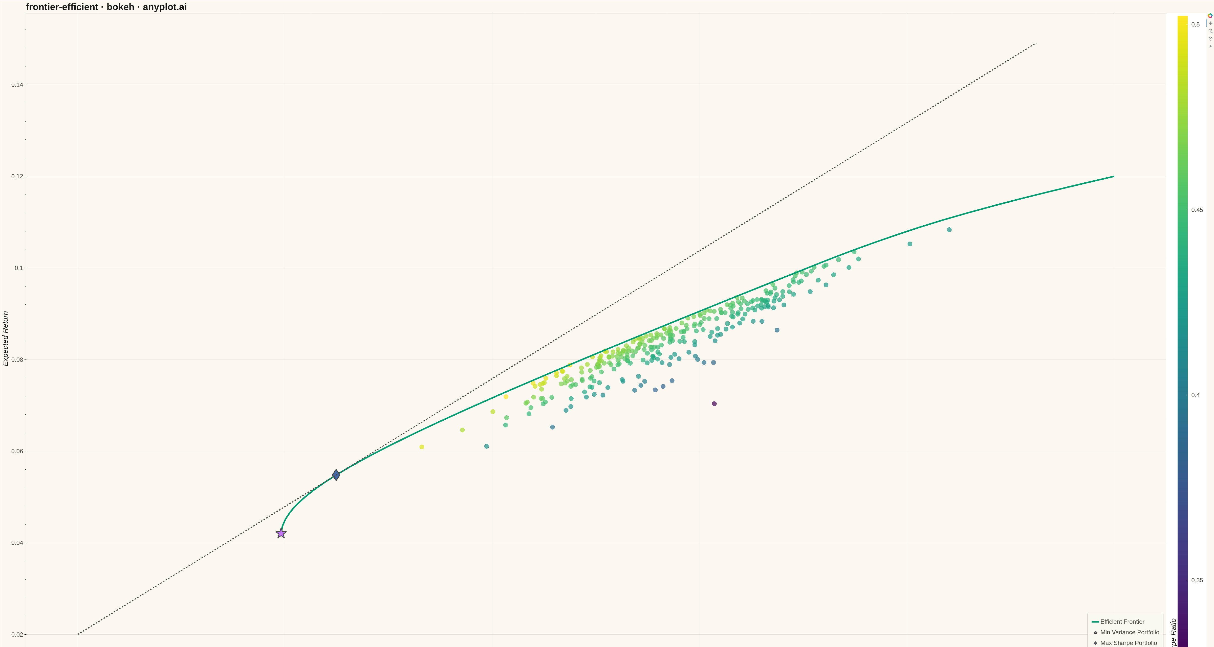
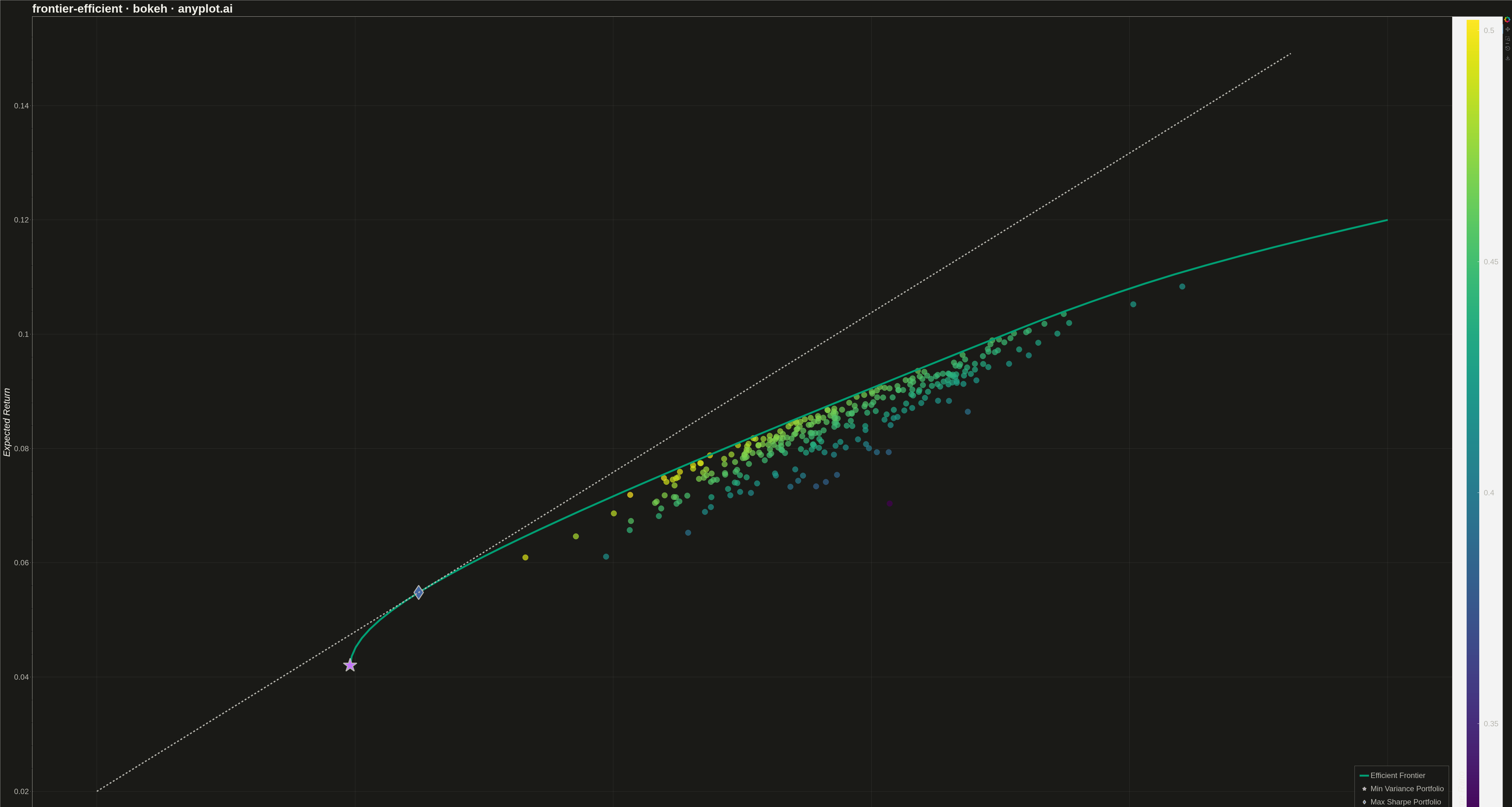
The efficient frontier is a fundamental visualization in Modern Portfolio Theory (MPT) that displays a curve of optimal portfolios offering the highest expected return for each level of risk (standard deviation). Portfolios on the frontier are "efficient" because no other portfolio exists with higher return for the same risk, or lower risk for the same return. This plot is essential for asset allocation decisions and understanding the risk-return tradeoff in investment portfolios.
""" anyplot.ai
frontier-efficient: Efficient Frontier for Portfolio Optimization
Library: bokeh 3.9.0 | Python 3.13.13
Quality: 90/100 | Updated: 2026-05-17
"""

import os
import sys
import time
from pathlib import Path


# Fix for running script named bokeh.py (avoid shadowing the bokeh package)
if Path(__file__).name == "bokeh.py":
    sys.path = [p for p in sys.path if Path(__file__).parent != Path(p)]

import numpy as np
from bokeh.io import output_file, save
from bokeh.models import ColorBar, ColumnDataSource, LinearColorMapper
from bokeh.palettes import Viridis256
from bokeh.plotting import figure
from scipy.optimize import minimize
from selenium import webdriver
from selenium.webdriver.chrome.options import Options


# Theme tokens
THEME = os.getenv("ANYPLOT_THEME", "light")
PAGE_BG = "#FAF8F1" if THEME == "light" else "#1A1A17"
INK = "#1A1A17" if THEME == "light" else "#F0EFE8"
INK_SOFT = "#4A4A44" if THEME == "light" else "#B8B7B0"
BRAND = "#009E73"  # Okabe-Ito position 1
ACCENT_1 = "#C475FD"  # Okabe-Ito position 2
ACCENT_2 = "#4467A3"  # Okabe-Ito position 3

# Asset data (5 assets)
np.random.seed(42)
n_assets = 5

expected_returns = np.array([0.04, 0.10, 0.12, 0.09, 0.07])

volatilities = np.array([0.05, 0.18, 0.25, 0.20, 0.22])
correlations = np.array(
    [
        [1.00, 0.20, 0.15, 0.10, 0.05],
        [0.20, 1.00, 0.85, 0.70, 0.30],
        [0.15, 0.85, 1.00, 0.65, 0.35],
        [0.10, 0.70, 0.65, 1.00, 0.40],
        [0.05, 0.30, 0.35, 0.40, 1.00],
    ]
)
cov_matrix = np.outer(volatilities, volatilities) * correlations
risk_free_rate = 0.02

# Generate random portfolios
n_portfolios = 300
portfolio_returns = []
portfolio_risks = []
portfolio_sharpes = []

for _ in range(n_portfolios):
    weights = np.random.random(n_assets)
    weights /= weights.sum()

    ret = np.dot(weights, expected_returns)
    risk = np.sqrt(np.dot(weights.T, np.dot(cov_matrix, weights)))
    sharpe = (ret - risk_free_rate) / risk

    portfolio_returns.append(ret)
    portfolio_risks.append(risk)
    portfolio_sharpes.append(sharpe)

portfolio_returns = np.array(portfolio_returns)
portfolio_risks = np.array(portfolio_risks)
portfolio_sharpes = np.array(portfolio_sharpes)

# Calculate efficient frontier using scipy optimization
constraints = {"type": "eq", "fun": lambda x: np.sum(x) - 1}
bounds = tuple((0, 1) for _ in range(n_assets))
init_weights = np.array([1 / n_assets] * n_assets)

# Find minimum variance portfolio
min_var_result = minimize(
    lambda w: np.sqrt(np.dot(w.T, np.dot(cov_matrix, w))),
    init_weights,
    method="SLSQP",
    bounds=bounds,
    constraints=constraints,
)
min_var_weights = min_var_result.x
min_var_return = np.dot(min_var_weights, expected_returns)
min_var_risk = np.sqrt(np.dot(min_var_weights.T, np.dot(cov_matrix, min_var_weights)))

# Find maximum Sharpe ratio portfolio
max_sharpe_result = minimize(
    lambda w: -(np.dot(w, expected_returns) - risk_free_rate) / np.sqrt(np.dot(w.T, np.dot(cov_matrix, w))),
    init_weights,
    method="SLSQP",
    bounds=bounds,
    constraints=constraints,
)
max_sharpe_weights = max_sharpe_result.x
max_sharpe_return = np.dot(max_sharpe_weights, expected_returns)
max_sharpe_risk = np.sqrt(np.dot(max_sharpe_weights.T, np.dot(cov_matrix, max_sharpe_weights)))
max_sharpe = (max_sharpe_return - risk_free_rate) / max_sharpe_risk

# Generate efficient frontier
frontier_returns = []
frontier_risks = []
target_returns = np.linspace(min_var_return, expected_returns.max(), 50)

for target in target_returns:
    constraints_ef = (
        {"type": "eq", "fun": lambda x: np.sum(x) - 1},
        {"type": "eq", "fun": lambda x, t=target: np.dot(x, expected_returns) - t},
    )
    result = minimize(
        lambda w: np.sqrt(np.dot(w.T, np.dot(cov_matrix, w))),
        init_weights,
        method="SLSQP",
        bounds=bounds,
        constraints=constraints_ef,
    )
    if result.success:
        frontier_returns.append(np.dot(result.x, expected_returns))
        frontier_risks.append(np.sqrt(np.dot(result.x.T, np.dot(cov_matrix, result.x))))

# Map Sharpe ratios to colors
sharpe_min = min(portfolio_sharpes)
sharpe_max = max(portfolio_sharpes)
sharpe_normalized = [(s - sharpe_min) / (sharpe_max - sharpe_min) for s in portfolio_sharpes]
color_indices = [int(s * 255) for s in sharpe_normalized]
colors = [Viridis256[min(i, 255)] for i in color_indices]

# Create ColumnDataSource
source = ColumnDataSource(
    data={"risk": portfolio_risks, "return": portfolio_returns, "sharpe": portfolio_sharpes, "color": colors}
)

# Create figure
p = figure(
    width=4800,
    height=2700,
    title="frontier-efficient · bokeh · anyplot.ai",
    x_axis_label="Risk (Standard Deviation)",
    y_axis_label="Expected Return",
    tools="pan,box_zoom,reset,save",
)

# Plot random portfolios with Sharpe ratio color coding
p.scatter("risk", "return", source=source, size=18, color="color", alpha=0.7)

# Plot efficient frontier curve
frontier_source = ColumnDataSource(data={"risk": frontier_risks, "return": frontier_returns})
p.line("risk", "return", source=frontier_source, line_width=6, color=BRAND, legend_label="Efficient Frontier")

# Mark minimum variance portfolio
min_var_source = ColumnDataSource(data={"risk": [min_var_risk], "return": [min_var_return]})
p.scatter(
    "risk",
    "return",
    source=min_var_source,
    size=45,
    color=ACCENT_1,
    marker="star",
    line_color=INK_SOFT,
    line_width=3,
    legend_label="Min Variance Portfolio",
)

# Mark maximum Sharpe ratio portfolio
max_sharpe_source = ColumnDataSource(data={"risk": [max_sharpe_risk], "return": [max_sharpe_return]})
p.scatter(
    "risk",
    "return",
    source=max_sharpe_source,
    size=45,
    color=ACCENT_2,
    marker="diamond",
    line_color=INK_SOFT,
    line_width=3,
    legend_label="Max Sharpe Portfolio",
)

# Capital Market Line (from risk-free rate tangent to max Sharpe portfolio)
cml_x_end = max(portfolio_risks) * 1.1
cml_y_end = risk_free_rate + max_sharpe * cml_x_end
cml_source = ColumnDataSource(data={"x": [0, cml_x_end], "y": [risk_free_rate, cml_y_end]})
p.line(
    "x", "y", source=cml_source, line_width=4, line_dash="dashed", color=INK_SOFT, legend_label="Capital Market Line"
)

# Style title and labels
p.title.text_font_size = "28pt"
p.title.text_color = INK
p.xaxis.axis_label_text_font_size = "22pt"
p.yaxis.axis_label_text_font_size = "22pt"
p.xaxis.axis_label_text_color = INK
p.yaxis.axis_label_text_color = INK
p.xaxis.major_label_text_font_size = "18pt"
p.yaxis.major_label_text_font_size = "18pt"
p.xaxis.major_label_text_color = INK_SOFT
p.yaxis.major_label_text_color = INK_SOFT

# Style grid
p.xgrid.grid_line_color = INK
p.ygrid.grid_line_color = INK
p.xgrid.grid_line_alpha = 0.10
p.ygrid.grid_line_alpha = 0.10

# Style legend (position bottom-right to avoid overlap)
p.legend.location = "bottom_right"
p.legend.label_text_font_size = "18pt"
p.legend.label_text_color = INK_SOFT
p.legend.background_fill_color = PAGE_BG
p.legend.background_fill_alpha = 0.9
p.legend.border_line_color = INK_SOFT
p.legend.glyph_height = 30
p.legend.glyph_width = 30
p.legend.spacing = 12
p.legend.padding = 15

# Add color bar for Sharpe ratio
color_mapper = LinearColorMapper(palette=Viridis256, low=sharpe_min, high=sharpe_max)
color_bar = ColorBar(
    color_mapper=color_mapper,
    title="Sharpe Ratio",
    title_text_font_size="22pt",
    major_label_text_font_size="18pt",
    label_standoff=15,
    width=40,
    location=(0, 0),
)
color_bar.title_text_color = INK
color_bar.major_label_text_color = INK_SOFT
p.add_layout(color_bar, "right")

# Set background and borders
p.background_fill_color = PAGE_BG
p.border_fill_color = PAGE_BG
p.outline_line_color = INK_SOFT
p.xaxis.axis_line_color = INK_SOFT
p.yaxis.axis_line_color = INK_SOFT
p.xaxis.major_tick_line_color = INK_SOFT
p.yaxis.major_tick_line_color = INK_SOFT
p.min_border_right = 120

# Save HTML
output_file(f"plot-{THEME}.html")
save(p)

# Screenshot with headless Chrome
W, H = 4800, 2700
opts = Options()
for arg in (
    "--headless=new",
    "--no-sandbox",
    "--disable-dev-shm-usage",
    "--disable-gpu",
    f"--window-size={W},{H}",
    "--hide-scrollbars",
):
    opts.add_argument(arg)
driver = webdriver.Chrome(options=opts)
driver.set_window_size(W, H)
driver.get(f"file://{Path(f'plot-{THEME}.html').resolve()}")
time.sleep(3)
driver.save_screenshot(f"plot-{THEME}.png")
driver.quit()
Runnable source as JSON, for any HTTP client: https://api.anyplot.ai/specs/frontier-efficient/bokeh/code. Any spec id and library id listed in llms-full.txt fit the same URL shape; every URL below is complete and callable.
{
  "spec_id": "frontier-efficient",
  "language": "python",
  "library": "bokeh",
  "page": "https://anyplot.ai/frontier-efficient/python/bokeh",
  "hub": "https://anyplot.ai/frontier-efficient",
  "code_json": "https://api.anyplot.ai/specs/frontier-efficient/bokeh/code",
  "spec_json": "https://api.anyplot.ai/specs/frontier-efficient",
  "render_light_png": "https://storage.googleapis.com/anyplot-images/plots/frontier-efficient/python/bokeh/plot-light.png",
  "render_dark_png": "https://storage.googleapis.com/anyplot-images/plots/frontier-efficient/python/bokeh/plot-dark.png",
  "interactive_light_html": "https://storage.googleapis.com/anyplot-images/plots/frontier-efficient/python/bokeh/plot-light.html",
  "interactive_dark_html": "https://storage.googleapis.com/anyplot-images/plots/frontier-efficient/python/bokeh/plot-dark.html",
  "quality_score": 90.0,
  "license": "MIT",
  "guide": "https://anyplot.ai/llms.txt"
}
Part of Efficient Frontier for Portfolio Optimization on anyplot.ai.