The same plot in 14 other libraries — Python: Altair, Bokeh, lets-plot, Matplotlib, Plotly, plotnine, Pygal, Seaborn; R: ggplot2; JavaScript: Chart.js, D3.js, Apache ECharts, Highcharts, MUI X Charts. Compare all 15 side by side: Efficient Frontier for Portfolio Optimization in Python, R, Julia and JavaScript.
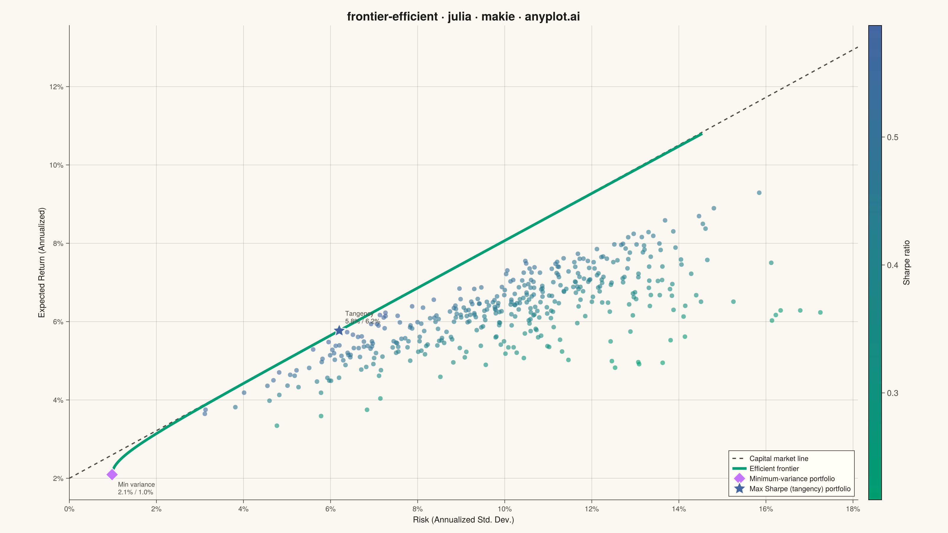
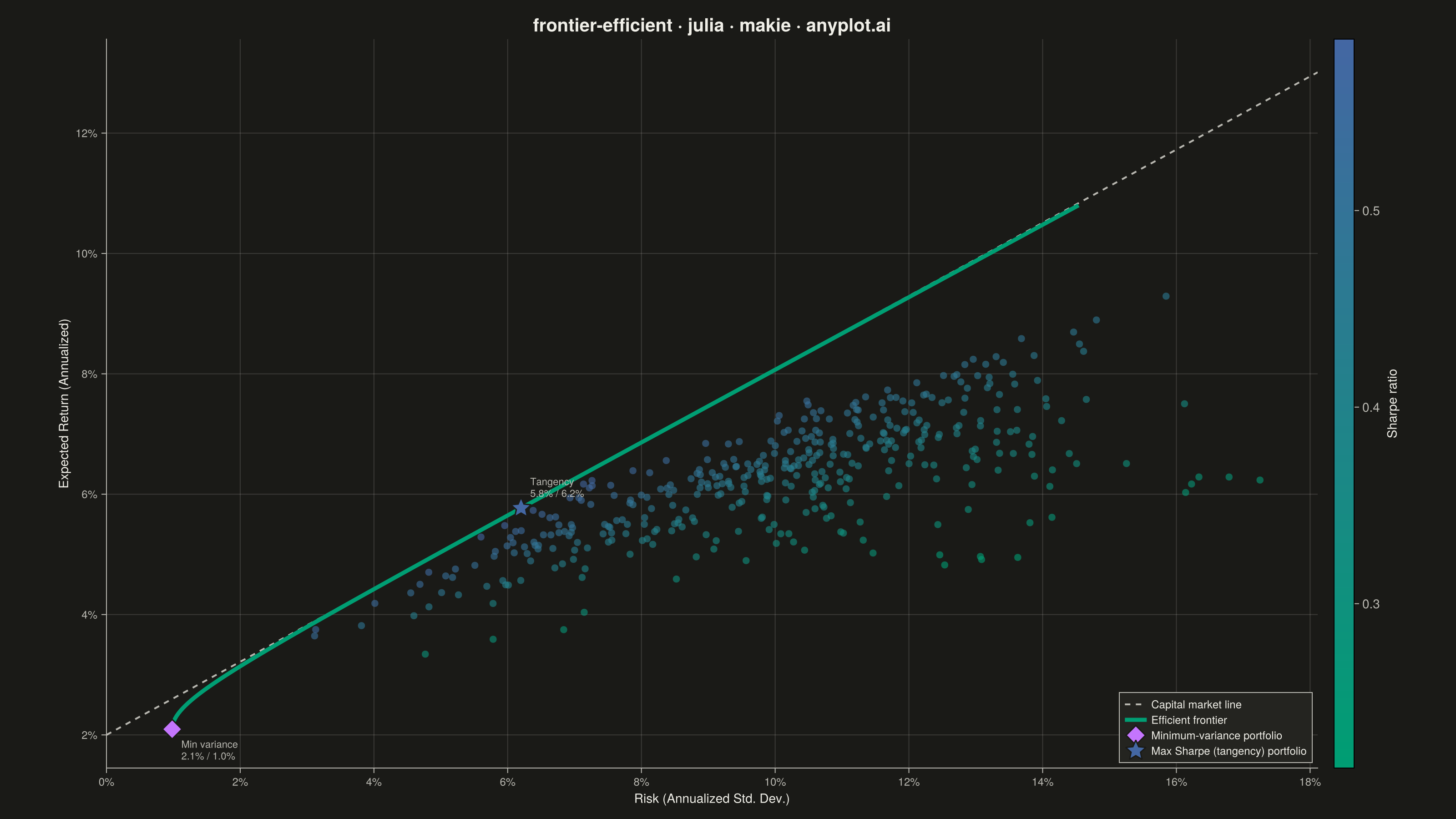
The efficient frontier is a fundamental visualization in Modern Portfolio Theory (MPT) that displays a curve of optimal portfolios offering the highest expected return for each level of risk (standard deviation). Portfolios on the frontier are "efficient" because no other portfolio exists with higher return for the same risk, or lower risk for the same return. This plot is essential for asset allocation decisions and understanding the risk-return tradeoff in investment portfolios.
# anyplot.ai
# frontier-efficient: Efficient Frontier for Portfolio Optimization
# Library: makie 0.21.9 | Julia 1.11.9
# Quality: 91/100 | Created: 2026-09-02

using CairoMakie
using Colors
using Random
using LinearAlgebra

Random.seed!(42)

# --- Theme tokens -----------------------------------------------------------
const THEME    = get(ENV, "ANYPLOT_THEME", "light")
const PAGE_BG  = THEME == "light" ? colorant"#FAF8F1" : colorant"#1A1A17"
const INK      = THEME == "light" ? colorant"#1A1A17" : colorant"#F0EFE8"
const INK_SOFT = THEME == "light" ? colorant"#4A4A44" : colorant"#B8B7B0"
const ELEVATED_BG = THEME == "light" ? colorant"#FFFDF6" : colorant"#242420"
const IMPRINT_PALETTE = [
    colorant"#009E73", colorant"#C475FD", colorant"#4467A3", colorant"#BD8233",
    colorant"#AE3030", colorant"#2ABCCD", colorant"#954477", colorant"#99B314",
]
const BRAND = IMPRINT_PALETTE[1]
const ANYPLOT_SEQ = cgrad([colorant"#009E73", colorant"#4467A3"])

# --- Asset universe (6-asset allocation, annualized figures) ---------------
assets = ["US Equities", "Intl Equities", "Corp Bonds", "Real Estate", "Commodities", "Cash"]
n_assets = length(assets)

expected_return = [0.10, 0.085, 0.04, 0.075, 0.055, 0.02]
volatility       = [0.18, 0.20, 0.06, 0.16, 0.22, 0.01]
risk_free_rate   = 0.02

# Single-factor correlation model: rho_ij = beta_i * beta_j (i != j), 1 on
# the diagonal. Guarantees a valid positive-definite correlation matrix as
# long as every |beta| < 1.
market_beta = [0.75, 0.70, -0.10, 0.60, 0.35, 0.0]
correlation = market_beta * market_beta' + Diagonal(1 .- market_beta .^ 2)
covariance = Diagonal(volatility) * correlation * Diagonal(volatility)

# --- Random simulated portfolios (long-only, weights sum to 1) --------------
n_portfolios = 400
sim_risk = zeros(n_portfolios)
sim_return = zeros(n_portfolios)
sim_sharpe = zeros(n_portfolios)

for i in 1:n_portfolios
    raw = -log.(rand(n_assets))          # exponential draws
    w = raw ./ sum(raw)                  # uniform on the simplex
    port_return = dot(w, expected_return)
    port_var = w' * covariance * w
    port_risk = sqrt(port_var)
    sim_return[i] = port_return
    sim_risk[i] = port_risk
    sim_sharpe[i] = (port_return - risk_free_rate) / port_risk
end

# --- Analytic efficient frontier (unconstrained mean-variance, closed form) -
cov_inv = inv(covariance)
ones_vec = ones(n_assets)
A = ones_vec' * cov_inv * ones_vec
B = ones_vec' * cov_inv * expected_return
C = expected_return' * cov_inv * expected_return
D = A * C - B^2

min_var_return = B / A
min_var_risk = sqrt(1 / A)

frontier_return = range(min_var_return, maximum(expected_return) * 1.08; length = 200)
frontier_variance = (A .* frontier_return .^ 2 .- 2 .* B .* frontier_return .+ C) ./ D
frontier_risk = sqrt.(frontier_variance)

# Tangency (maximum Sharpe ratio) portfolio
tangency_raw = cov_inv * (expected_return .- risk_free_rate)
tangency_weights = tangency_raw ./ sum(tangency_raw)
tangency_return = dot(tangency_weights, expected_return)
tangency_risk = sqrt(tangency_weights' * covariance * tangency_weights)

# Capital market line: from the risk-free rate through the tangency portfolio
max_risk_axis = max(maximum(sim_risk), maximum(frontier_risk)) * 1.05
cml_risk = [0.0, max_risk_axis]
cml_return = risk_free_rate .+ (tangency_return - risk_free_rate) / tangency_risk .* cml_risk

# --- Plot --------------------------------------------------------------------
pct_format(values) = [string(round(Int, v * 100), "%") for v in values]

# Explicit round-number tick steps (2 pp) so labels land on clean integers
# instead of rounding arbitrary auto-ticks to the nearest percent.
xtick_step = 0.02
ytick_step = 0.02
xtick_vals = 0:xtick_step:(ceil(max_risk_axis / xtick_step) * xtick_step)
ytick_lo = floor(min_var_return / ytick_step) * ytick_step
ytick_hi = ceil(maximum(frontier_return) / ytick_step) * ytick_step
ytick_vals = ytick_lo:ytick_step:ytick_hi

fig = Figure(
    size            = (1600, 900),
    fontsize        = 14,
    backgroundcolor = PAGE_BG,
)

ax = Axis(
    fig[1, 1];
    title              = "frontier-efficient · julia · makie · anyplot.ai",
    titlesize          = 20,
    titlecolor         = INK,
    xlabel             = "Risk (Annualized Std. Dev.)",
    ylabel             = "Expected Return (Annualized)",
    xlabelsize         = 14,
    ylabelsize         = 14,
    xlabelcolor        = INK,
    ylabelcolor        = INK,
    xticklabelsize     = 12,
    yticklabelsize     = 12,
    xticklabelcolor    = INK_SOFT,
    yticklabelcolor    = INK_SOFT,
    xtickcolor         = INK_SOFT,
    ytickcolor         = INK_SOFT,
    xticks             = xtick_vals,
    yticks             = ytick_vals,
    xtickformat        = pct_format,
    ytickformat        = pct_format,
    backgroundcolor    = PAGE_BG,
    topspinevisible    = false,
    rightspinevisible  = false,
    leftspinecolor     = INK_SOFT,
    bottomspinecolor   = INK_SOFT,
    xgridcolor         = RGBAf(INK.r, INK.g, INK.b, 0.15),
    ygridcolor         = RGBAf(INK.r, INK.g, INK.b, 0.15),
    xminorgridvisible  = false,
    yminorgridvisible  = false,
)
xlims!(ax, 0, max_risk_axis)

scatter!(
    ax, sim_risk, sim_return;
    color = sim_sharpe, colormap = ANYPLOT_SEQ,
    colorrange = (minimum(sim_sharpe), maximum(sim_sharpe)),
    markersize = 11, alpha = 0.6, strokewidth = 0,
)

lines!(ax, cml_risk, cml_return; color = INK_SOFT, linewidth = 2, linestyle = :dash, label = "Capital market line")
lines!(ax, frontier_risk, collect(frontier_return); color = BRAND, linewidth = 4.5, label = "Efficient frontier")

scatter!(
    ax, [min_var_risk], [min_var_return];
    color = IMPRINT_PALETTE[2], marker = :diamond, markersize = 24,
    strokewidth = 1.5, strokecolor = PAGE_BG, label = "Minimum-variance portfolio",
)
scatter!(
    ax, [tangency_risk], [tangency_return];
    color = IMPRINT_PALETTE[3], marker = :star5, markersize = 26,
    strokewidth = 1.5, strokecolor = PAGE_BG, label = "Max Sharpe (tangency) portfolio",
)

# Small callouts so the two key portfolios' return/risk are legible at a glance
callout(v) = string(round(v * 100, digits = 1), "%")
text!(
    ax, min_var_risk, min_var_return;
    text = "Min variance\n$(callout(min_var_return)) / $(callout(min_var_risk))",
    color = INK_SOFT, fontsize = 11, align = (:left, :top), offset = (10, -10),
)
text!(
    ax, tangency_risk, tangency_return;
    text = "Tangency\n$(callout(tangency_return)) / $(callout(tangency_risk))",
    color = INK_SOFT, fontsize = 11, align = (:left, :bottom), offset = (10, 10),
)

Colorbar(
    fig[1, 2];
    limits = (minimum(sim_sharpe), maximum(sim_sharpe)),
    colormap = ANYPLOT_SEQ,
    label = "Sharpe ratio",
    labelcolor = INK,
    ticklabelcolor = INK_SOFT,
    tickcolor = INK_SOFT,
    width = 22,
)

axislegend(
    ax; position = :rb, framevisible = true,
    backgroundcolor = ELEVATED_BG, framecolor = INK_SOFT,
    labelcolor = INK, labelsize = 12, patchsize = (24, 12),
)

colsize!(fig.layout, 1, Relative(0.92))

# --- Save ---------------------------------------------------------------------
save("plot-$(THEME).png", fig; px_per_unit = 2)
Runnable source as JSON, for any HTTP client: https://api.anyplot.ai/specs/frontier-efficient/makie/code. Any spec id and library id listed in llms-full.txt fit the same URL shape; every URL below is complete and callable.
{
  "spec_id": "frontier-efficient",
  "language": "julia",
  "library": "makie",
  "page": "https://anyplot.ai/frontier-efficient/julia/makie",
  "hub": "https://anyplot.ai/frontier-efficient",
  "code_json": "https://api.anyplot.ai/specs/frontier-efficient/makie/code",
  "spec_json": "https://api.anyplot.ai/specs/frontier-efficient",
  "render_light_png": "https://storage.googleapis.com/anyplot-images/plots/frontier-efficient/julia/makie/plot-light.png",
  "render_dark_png": "https://storage.googleapis.com/anyplot-images/plots/frontier-efficient/julia/makie/plot-dark.png",
  "quality_score": 91.0,
  "license": "MIT",
  "guide": "https://anyplot.ai/llms.txt"
}
Part of Efficient Frontier for Portfolio Optimization on anyplot.ai.