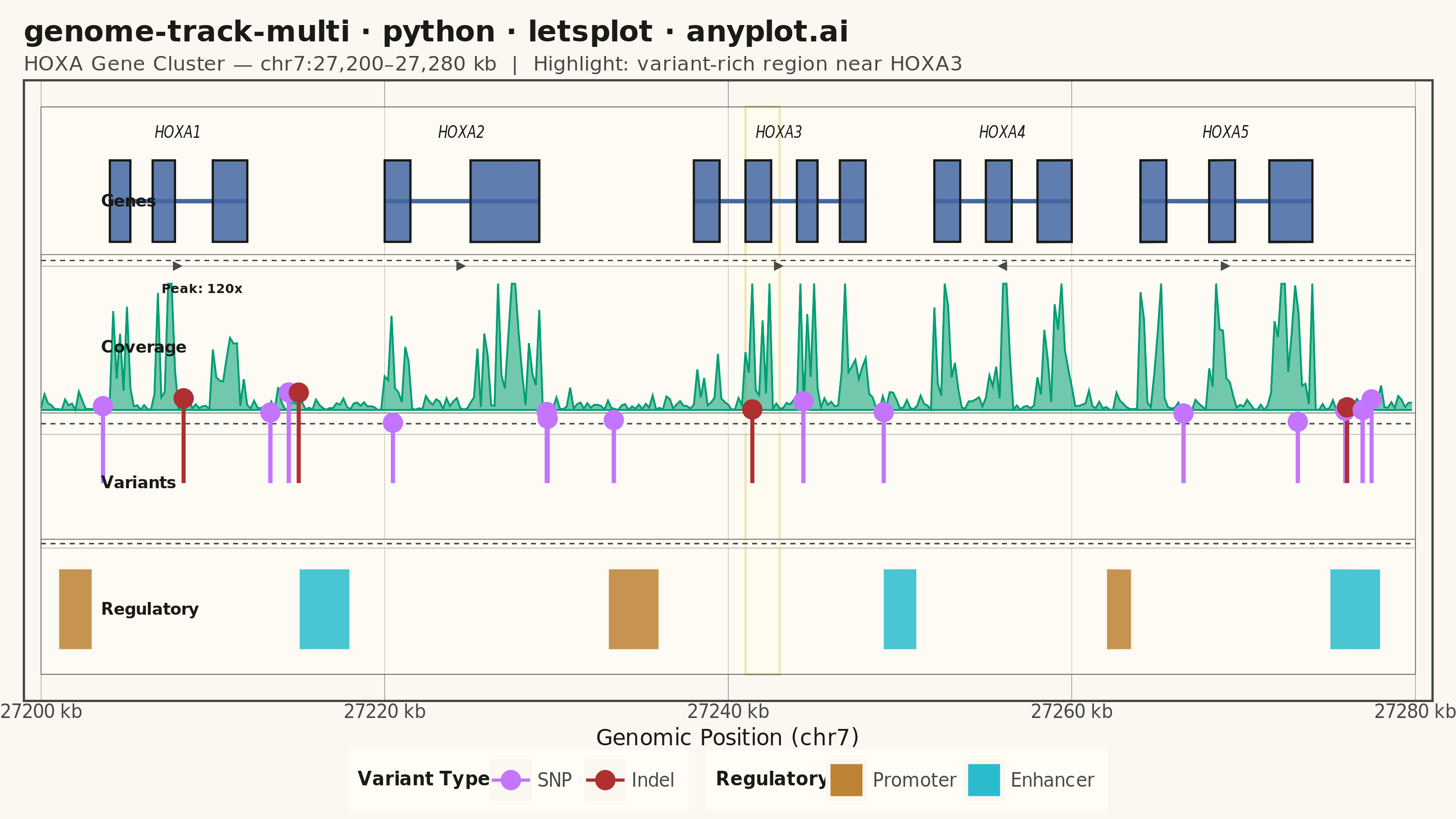
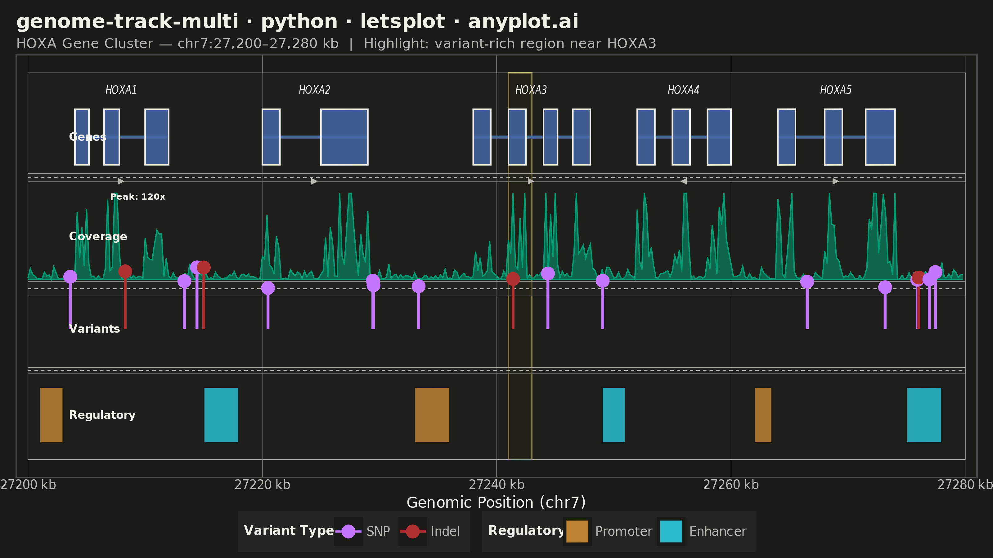
A multi-track genome browser view that displays different types of genomic data aligned along a shared chromosomal coordinate axis. Multiple parallel horizontal tracks (gene annotations, read coverage, variants, regulatory elements) are stacked vertically, each showing a different data type at the same genomic locus. This visualization is essential for integrative genomics, enabling researchers to explore relationships between gene structure, expression, variation, and regulation in a single coordinated view.
""" anyplot.ai
genome-track-multi: Genome Track Viewer
Library: letsplot 4.10.1 | Python 3.13.13
Quality: 86/100 | Updated: 2026-06-02
"""

import os

import numpy as np
import pandas as pd
from lets_plot import *


LetsPlot.setup_html()

# Theme-adaptive chrome tokens (Imprint palette)
THEME = os.getenv("ANYPLOT_THEME", "light")
PAGE_BG = "#FAF8F1" if THEME == "light" else "#1A1A17"
ELEVATED_BG = "#FFFDF6" if THEME == "light" else "#242420"
INK = "#1A1A17" if THEME == "light" else "#F0EFE8"
INK_SOFT = "#4A4A44" if THEME == "light" else "#B8B7B0"
INK_MUTED = "#6B6A63" if THEME == "light" else "#A8A79F"

# Imprint categorical palette
IMPRINT = ["#009E73", "#C475FD", "#4467A3", "#BD8233", "#AE3030", "#2ABCCD", "#954477", "#99B314"]
AMBER = "#DDCC77"

np.random.seed(42)

# Genomic region: chr7:27,200,000-27,280,000 (HOXA gene cluster)
chrom = "chr7"
region_start = 27200000
region_end = 27280000

# Track 1: Gene annotations
genes = pd.DataFrame(
    {
        "name": ["HOXA1", "HOXA2", "HOXA3", "HOXA4", "HOXA5"],
        "start": [27204000, 27220000, 27238000, 27252000, 27264000],
        "end": [27212000, 27229000, 27248000, 27260000, 27274000],
        "strand": ["+", "+", "+", "-", "+"],
    }
)

# Exons within each gene
exons = pd.DataFrame(
    {
        "gene": [
            "HOXA1",
            "HOXA1",
            "HOXA1",
            "HOXA2",
            "HOXA2",
            "HOXA3",
            "HOXA3",
            "HOXA3",
            "HOXA3",
            "HOXA4",
            "HOXA4",
            "HOXA4",
            "HOXA5",
            "HOXA5",
            "HOXA5",
        ],
        "start": [
            27204000,
            27206500,
            27210000,
            27220000,
            27225000,
            27238000,
            27241000,
            27244000,
            27246500,
            27252000,
            27255000,
            27258000,
            27264000,
            27268000,
            27271500,
        ],
        "end": [
            27205200,
            27207800,
            27212000,
            27221500,
            27229000,
            27239500,
            27242500,
            27245200,
            27248000,
            27253500,
            27256500,
            27260000,
            27265500,
            27269500,
            27274000,
        ],
    }
)

# Track 2: Coverage — simulated RNA-seq read depth
coverage_positions = np.arange(region_start, region_end, 200)
base_coverage = np.random.exponential(5, len(coverage_positions))
for _, exon in exons.iterrows():
    mask = (coverage_positions >= exon["start"]) & (coverage_positions <= exon["end"])
    base_coverage[mask] += np.random.exponential(40, mask.sum())
coverage_df = pd.DataFrame({"position": coverage_positions, "depth": np.clip(base_coverage, 0, 120)})

# Track 3: Variants (SNPs and indels)
variant_positions = np.sort(np.random.choice(range(region_start + 1000, region_end - 1000), size=18, replace=False))
variant_types = np.random.choice(["SNP", "SNP", "SNP", "Indel"], size=18)
variant_quality = np.random.uniform(20, 99, size=18)
variants_df = pd.DataFrame({"position": variant_positions, "type": variant_types, "quality": variant_quality})

# Track 4: Regulatory elements
regulatory = pd.DataFrame(
    {
        "start": [27201000, 27215000, 27233000, 27249000, 27262000, 27275000],
        "end": [27203000, 27218000, 27236000, 27251000, 27263500, 27278000],
        "element": ["Promoter", "Enhancer", "Promoter", "Enhancer", "Promoter", "Enhancer"],
    }
)

# Track layout
tracks = {
    "Genes": {"center": 4.2, "half_h": 0.42, "pad_bot": 0.25, "pad_top": 0.55},
    "Coverage": {"center": 2.7, "half_h": 0.65, "pad_bot": 0.25, "pad_top": 0.30},
    "Variants": {"center": 1.3, "half_h": 0.42, "pad_bot": 0.25, "pad_top": 0.30},
    "Regulatory": {"center": 0.0, "half_h": 0.42, "pad_bot": 0.25, "pad_top": 0.30},
}

scale = 1000.0
x_start = region_start / scale
x_end = region_end / scale

# Gene track data
t = tracks["Genes"]
gene_intron_df = pd.DataFrame(
    {"x": genes["start"] / scale, "xend": genes["end"] / scale, "y": t["center"], "yend": t["center"]}
)
exon_df = pd.DataFrame(
    {
        "xmin": exons["start"] / scale,
        "xmax": exons["end"] / scale,
        "ymin": t["center"] - t["half_h"],
        "ymax": t["center"] + t["half_h"],
        "gene": exons["gene"],
    }
)
exon_df["exon_size"] = ((exons["end"] - exons["start"]) / 1000).round(1).astype(str) + " kb"
gene_label_df = pd.DataFrame(
    {"x": (genes["start"] + genes["end"]) / 2 / scale, "y": t["center"] + t["half_h"] + 0.28, "label": genes["name"]}
)
strand_arrows = []
for _, g in genes.iterrows():
    mid = (g["start"] + g["end"]) / 2 / scale
    arrow_char = "▶" if g["strand"] == "+" else "◀"
    strand_arrows.append({"x": mid, "y": t["center"] - t["half_h"] - 0.24, "label": arrow_char})
strand_df = pd.DataFrame(strand_arrows)

# Coverage track data
t = tracks["Coverage"]
cov_plot_df = coverage_df.copy()
cov_plot_df["x"] = cov_plot_df["position"] / scale
max_depth = cov_plot_df["depth"].max()
cov_plot_df["y"] = t["center"] - t["half_h"] + (cov_plot_df["depth"] / max_depth) * (2 * t["half_h"])
cov_plot_df["ybase"] = t["center"] - t["half_h"]
cov_plot_df["depth_label"] = cov_plot_df["depth"].round(1).astype(str) + "x"
cov_plot_df["pos_label"] = (cov_plot_df["position"] / 1000).round(1).astype(str) + " kb"

# Variant track data
t = tracks["Variants"]
var_plot_df = variants_df.copy()
var_plot_df["x"] = var_plot_df["position"] / scale
var_plot_df["y_base"] = t["center"]
min_stem = 0.5  # raised from 0.3 — improves low-quality variant visibility
max_stem = 2 * t["half_h"] + 0.15
var_plot_df["y_top"] = t["center"] + min_stem * max_stem + (var_plot_df["quality"] / 100) * (1 - min_stem) * max_stem
var_plot_df["qual_label"] = "QUAL: " + var_plot_df["quality"].round(1).astype(str)
var_plot_df["pos_label"] = (var_plot_df["position"] / 1000).round(1).astype(str) + " kb"

# Regulatory track data
t = tracks["Regulatory"]
reg_plot_df = pd.DataFrame(
    {
        "xmin": regulatory["start"] / scale,
        "xmax": regulatory["end"] / scale,
        "ymin": t["center"] - t["half_h"],
        "ymax": t["center"] + t["half_h"],
        "element": regulatory["element"],
        "size_label": ((regulatory["end"] - regulatory["start"]) / 1000).round(1).astype(str) + " kb",
    }
)

# Track background shading (alternating light/dark)
bg_rows = []
for name, t in tracks.items():
    bg_rows.append(
        {
            "xmin": x_start,
            "xmax": x_end,
            "ymin": t["center"] - t["half_h"] - t["pad_bot"],
            "ymax": t["center"] + t["half_h"] + t["pad_top"],
            "track": name,
        }
    )
track_bg = pd.DataFrame(bg_rows)

# Divider lines
track_order = ["Regulatory", "Variants", "Coverage", "Genes"]
divider_positions = []
for i in range(len(track_order) - 1):
    lo = tracks[track_order[i]]
    hi = tracks[track_order[i + 1]]
    y_mid = (lo["center"] + lo["half_h"] + lo["pad_top"] + hi["center"] - hi["half_h"] - hi["pad_bot"]) / 2
    divider_positions.append(y_mid)
divider_df = pd.DataFrame({"x": [x_start] * 3, "xend": [x_end] * 3, "y": divider_positions, "yend": divider_positions})

# Track labels shifted right to clear leftmost data elements
track_labels_df = pd.DataFrame(
    {"x": [x_start + 3.5] * 4, "y": [tracks[n]["center"] for n in track_order], "label": track_order}
)

# Highlight region: variant-dense area near HOXA3
highlight_df = pd.DataFrame(
    {
        "xmin": [27241.0],
        "xmax": [27243.0],
        "ymin": [tracks["Regulatory"]["center"] - tracks["Regulatory"]["half_h"] - tracks["Regulatory"]["pad_bot"]],
        "ymax": [tracks["Genes"]["center"] + tracks["Genes"]["half_h"] + tracks["Genes"]["pad_top"]],
    }
)

# Peak coverage annotation
peak_idx = cov_plot_df["depth"].idxmax()
peak_x = cov_plot_df.loc[peak_idx, "x"]
peak_depth = cov_plot_df.loc[peak_idx, "depth"]
t = tracks["Coverage"]
peak_annotation_df = pd.DataFrame(
    {"x": [peak_x + 2.0], "y": [t["center"] + t["half_h"] - 0.05], "label": [f"Peak: {peak_depth:.0f}x"]}
)

# Colors — Imprint palette assignments (fixes green/red colorblind pair)
exon_color = IMPRINT[2]  # #4467A3 blue — gene exons (structural)
cov_fill = IMPRINT[0]  # #009E73 green — coverage (first categorical series)
snp_color = IMPRINT[1]  # #C475FD lavender — SNP
indel_color = IMPRINT[4]  # #AE3030 red — Indel (semantic bad/error)
promoter_color = IMPRINT[3]  # #BD8233 ochre — Promoter (replaces green, fixes colorblind issue)
enhancer_color = IMPRINT[5]  # #2ABCCD cyan — Enhancer

# Highlight colors: amber (theme-independent warning/focus)
highlight_fill = "#FFF8E1" if THEME == "light" else "#2A2000"
highlight_border = AMBER

tick_positions = list(range(int(x_start), int(x_end) + 1, 20))
tick_labels = [f"{v} kb" for v in tick_positions]

# Title: genome-track-multi · python · letsplot · anyplot.ai  (51 chars < 67 baseline, no scaling needed)
title_str = "genome-track-multi · python · letsplot · anyplot.ai"

plot = (
    ggplot()
    # Highlight region
    + geom_rect(
        aes(xmin="xmin", xmax="xmax", ymin="ymin", ymax="ymax"),
        data=highlight_df,
        fill=highlight_fill,
        color=highlight_border,
        size=0.5,
        alpha=0.4,
    )
    # Track background shading
    + geom_rect(
        aes(xmin="xmin", xmax="xmax", ymin="ymin", ymax="ymax"),
        data=track_bg,
        fill=ELEVATED_BG,
        color=INK_MUTED,
        size=0.2,
        alpha=0.5,
    )
    # Divider lines
    + geom_segment(
        aes(x="x", xend="xend", y="y", yend="yend"), data=divider_df, color=INK_SOFT, size=0.3, linetype="dashed"
    )
    # Gene track: intron lines
    + geom_segment(aes(x="x", xend="xend", y="y", yend="yend"), data=gene_intron_df, color=exon_color, size=1.0)
    # Gene track: exon rectangles
    + geom_rect(
        aes(xmin="xmin", xmax="xmax", ymin="ymin", ymax="ymax"),
        data=exon_df,
        fill=exon_color,
        color=INK,
        size=0.5,
        alpha=0.85,
        tooltips=layer_tooltips().line("Gene: @gene").line("Size: @exon_size"),
    )
    # Gene labels (italic, above exons)
    + geom_text(aes(x="x", y="y", label="label"), data=gene_label_df, size=4, color=INK, fontface="italic")
    # Strand direction arrows — size raised to 3.5 mm for legibility
    + geom_text(aes(x="x", y="y", label="label"), data=strand_df, size=3.5, color=INK_SOFT)
    # Coverage: filled area
    + geom_ribbon(
        aes(x="x", ymin="ybase", ymax="y"),
        data=cov_plot_df,
        fill=cov_fill,
        color=cov_fill,
        alpha=0.55,
        size=0.4,
        tooltips=layer_tooltips().line("Position: @pos_label").line("Depth: @depth_label"),
    )
    # Coverage peak annotation
    + geom_text(aes(x="x", y="y", label="label"), data=peak_annotation_df, size=3.5, color=INK, fontface="bold")
    # Variant lollipop stems
    + geom_segment(aes(x="x", xend="x", y="y_base", yend="y_top", color="type"), data=var_plot_df, size=1.0)
    # Variant lollipop heads
    + geom_point(
        aes(x="x", y="y_top", color="type"),
        data=var_plot_df,
        size=5,
        stroke=0.8,
        tooltips=layer_tooltips().line("@type").line("@qual_label").line("Position: @pos_label"),
    )
    # Regulatory elements
    + geom_rect(
        aes(xmin="xmin", xmax="xmax", ymin="ymin", ymax="ymax", fill="element"),
        data=reg_plot_df,
        alpha=0.85,
        size=0.4,
        color=PAGE_BG,
        tooltips=layer_tooltips().line("@element").line("Size: @size_label"),
    )
    # Track labels at center y — avoids overlap with gene names at top of Genes track
    + geom_text(aes(x="x", y="y", label="label"), data=track_labels_df, size=4.5, color=INK, fontface="bold", hjust=0)
    # Scales
    + scale_color_manual(values={"SNP": snp_color, "Indel": indel_color}, name="Variant Type")
    + scale_fill_manual(values={"Promoter": promoter_color, "Enhancer": enhancer_color}, name="Regulatory")
    + scale_x_continuous(
        name=f"Genomic Position ({chrom})", breaks=tick_positions, labels=tick_labels, expand=[0.01, 0.01]
    )
    + scale_y_continuous(expand=[0.04, 0.04])
    + labs(
        title=title_str,
        subtitle="HOXA Gene Cluster — chr7:27,200–27,280 kb  |  Highlight: variant-rich region near HOXA3",
    )
    + coord_cartesian(xlim=[x_start - 1, x_end + 1])
    + theme_minimal()
    + theme(
        plot_title=element_text(size=16, face="bold", color=INK),
        plot_subtitle=element_text(size=11, color=INK_SOFT),
        axis_title_x=element_text(size=12, color=INK),
        axis_title_y=element_blank(),
        axis_text_x=element_text(size=10, color=INK_SOFT, angle=0),
        axis_text_y=element_blank(),
        axis_ticks_y=element_blank(),
        panel_grid_major_x=element_line(color=INK_SOFT, size=0.15),
        panel_grid_major_y=element_blank(),
        panel_grid_minor=element_blank(),
        legend_title=element_text(size=10, face="bold", color=INK),
        legend_text=element_text(size=10, color=INK_SOFT),
        legend_background=element_rect(fill=ELEVATED_BG, color=INK_SOFT),
        legend_position="bottom",
        legend_box="horizontal",
        legend_direction="horizontal",
        plot_background=element_rect(fill=PAGE_BG, color=PAGE_BG),
        panel_background=element_rect(fill=PAGE_BG),
        plot_margin=[10, 10, 5, 10],
    )
    + ggsize(800, 450)
)

# Save — scale=4 → 3200×1800 px
ggsave(plot, f"plot-{THEME}.png", path=".", scale=4)
ggsave(plot, f"plot-{THEME}.html", path=".")
Runnable source as JSON, for any HTTP client: https://api.anyplot.ai/specs/genome-track-multi/letsplot/code. Any spec id and library id listed in llms-full.txt fit the same URL shape; every URL below is complete and callable.
{
  "spec_id": "genome-track-multi",
  "language": "python",
  "library": "letsplot",
  "page": "https://anyplot.ai/genome-track-multi/python/letsplot",
  "hub": "https://anyplot.ai/genome-track-multi",
  "code_json": "https://api.anyplot.ai/specs/genome-track-multi/letsplot/code",
  "spec_json": "https://api.anyplot.ai/specs/genome-track-multi",
  "render_light_png": "https://storage.googleapis.com/anyplot-images/plots/genome-track-multi/python/letsplot/plot-light.png",
  "render_dark_png": "https://storage.googleapis.com/anyplot-images/plots/genome-track-multi/python/letsplot/plot-dark.png",
  "interactive_light_html": "https://storage.googleapis.com/anyplot-images/plots/genome-track-multi/python/letsplot/plot-light.html",
  "interactive_dark_html": "https://storage.googleapis.com/anyplot-images/plots/genome-track-multi/python/letsplot/plot-dark.html",
  "quality_score": 86.0,
  "license": "MIT",
  "guide": "https://anyplot.ai/llms.txt"
}
Part of Genome Track Viewer on anyplot.ai.