The same plot in 14 other libraries — Python: Altair, Bokeh, lets-plot, Matplotlib, Plotly, plotnine, Pygal, Seaborn; Julia: Makie.jl; JavaScript: Chart.js, D3.js, Apache ECharts, Highcharts, MUI X Charts. Compare all 15 side by side: Genome Track Viewer in Python, R, Julia and JavaScript.
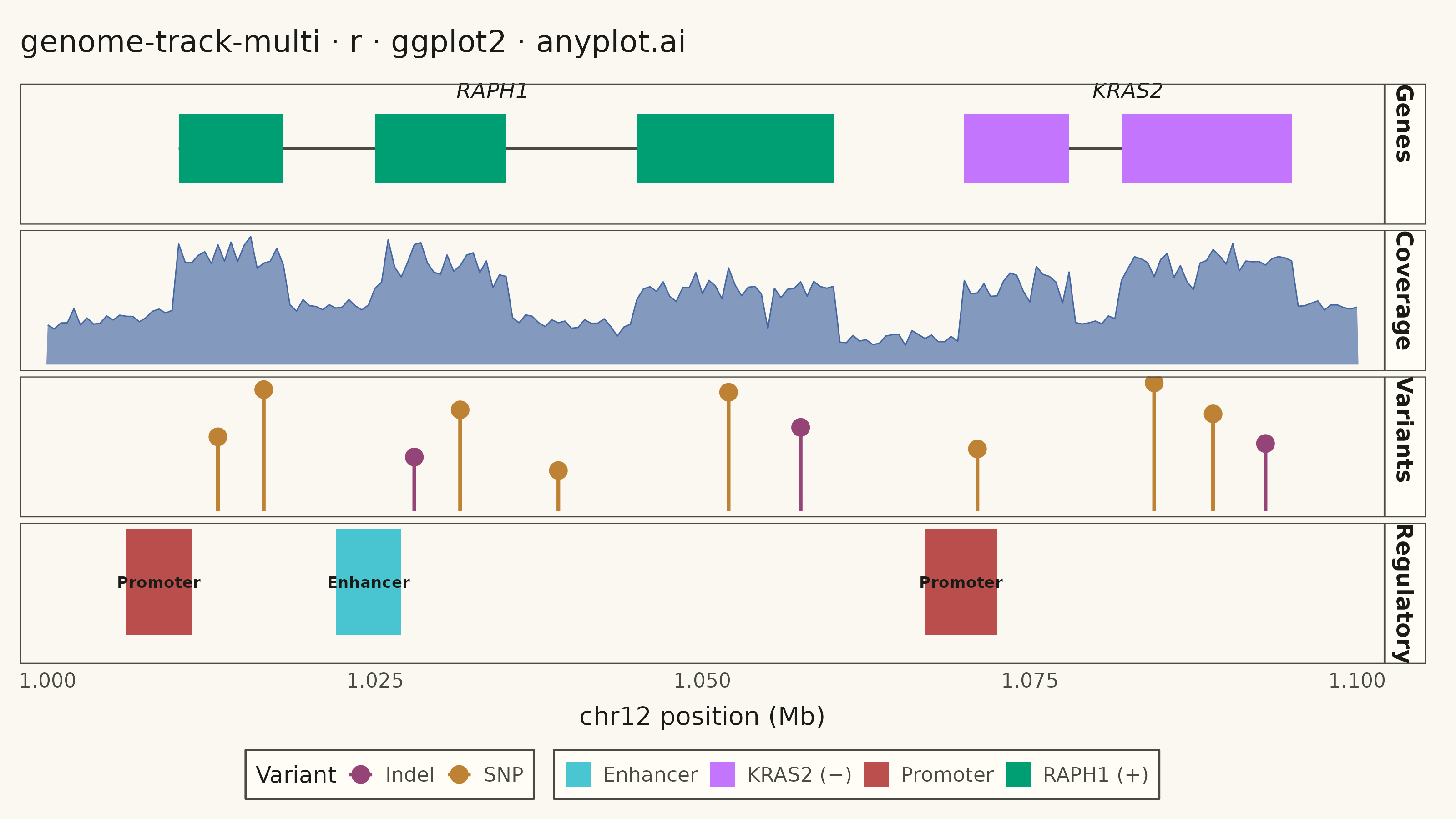
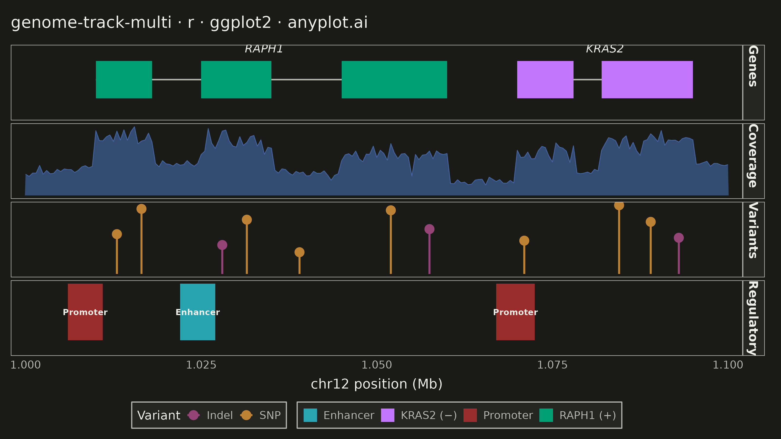
A multi-track genome browser view that displays different types of genomic data aligned along a shared chromosomal coordinate axis. Multiple parallel horizontal tracks (gene annotations, read coverage, variants, regulatory elements) are stacked vertically, each showing a different data type at the same genomic locus. This visualization is essential for integrative genomics, enabling researchers to explore relationships between gene structure, expression, variation, and regulation in a single coordinated view.
#' anyplot.ai
#' genome-track-multi: Genome Track Viewer
#' Library: ggplot2 3.5.1 | R 4.4.1
#' Quality: 89/100 | Created: 2026-06-02

library(ggplot2)
library(ragg)

set.seed(42)

# Theme tokens (Imprint palette — theme-adaptive chrome)
THEME       <- Sys.getenv("ANYPLOT_THEME", "light")
PAGE_BG     <- if (THEME == "light") "#FAF8F1" else "#1A1A17"
ELEVATED_BG <- if (THEME == "light") "#FFFDF6" else "#242420"
INK         <- if (THEME == "light") "#1A1A17" else "#F0EFE8"
INK_SOFT    <- if (THEME == "light") "#4A4A44" else "#B8B7B0"
INK_MUTED   <- if (THEME == "light") "#6B6A63" else "#A8A79F"

# Imprint categorical palette — hybrid-v3 sort, first series always #009E73
IMPRINT_PALETTE <- c(
  "#009E73",  # 1 brand green
  "#C475FD",  # 2 lavender
  "#4467A3",  # 3 blue
  "#BD8233",  # 4 ochre
  "#AE3030",  # 5 matte red
  "#2ABCCD",  # 6 cyan
  "#954477",  # 7 rose
  "#99B314"   # 8 lime
)

# Genomic region: chr12: 1,000,000 – 1,100,000 (100 kb window)
CHR          <- "chr12"
REGION_START <- 1000000L
REGION_END   <- 1100000L
TRACK_LEVELS <- c("Genes", "Coverage", "Variants", "Regulatory")

# --- Genes track data -------------------------------------------------------
# Two genes: RAPH1 (+ strand, 3 exons) and KRAS2 (− strand, 2 exons)
exons_df <- data.frame(
  xmin  = c(1010000, 1025000, 1045000, 1070000, 1082000),
  xmax  = c(1018000, 1035000, 1060000, 1078000, 1095000),
  ymin  = 0.25,
  ymax  = 0.75,
  gene  = c("RAPH1 (+)", "RAPH1 (+)", "RAPH1 (+)", "KRAS2 (−)", "KRAS2 (−)"),
  track = factor("Genes", levels = TRACK_LEVELS),
  stringsAsFactors = FALSE
)

gene_bodies <- data.frame(
  x     = c(1010000, 1070000),
  xend  = c(1060000, 1095000),
  y     = 0.5,
  yend  = 0.5,
  track = factor("Genes", levels = TRACK_LEVELS)
)

gene_labels <- data.frame(
  x     = c(1034000, 1082500),
  y     = 0.92,
  label = c("RAPH1", "KRAS2"),
  track = factor("Genes", levels = TRACK_LEVELS),
  stringsAsFactors = FALSE
)

# --- Coverage track data ----------------------------------------------------
cov_pos  <- seq(REGION_START, REGION_END, by = 500)
n_cov    <- length(cov_pos)
base_cov <- 80 + 35 * sin((cov_pos - REGION_START) /
                           (REGION_END - REGION_START) * pi * 2.5)

# Elevated depth over exonic regions (transcribed segments)
exon_boost <- numeric(n_cov)
exon_coords <- list(
  c(1010000, 1018000), c(1025000, 1035000), c(1045000, 1060000),
  c(1070000, 1078000), c(1082000, 1095000)
)
for (coords in exon_coords) {
  idx <- cov_pos >= coords[1] & cov_pos <= coords[2]
  exon_boost[idx] <- exon_boost[idx] + rnorm(sum(idx), mean = 90, sd = 20)
}

coverage_df <- data.frame(
  position = cov_pos,
  depth    = pmax(3, base_cov + exon_boost + rnorm(n_cov, 0, 8)),
  track    = factor("Coverage", levels = TRACK_LEVELS)
)

# --- Variants track data ----------------------------------------------------
variants_df <- data.frame(
  position = c(1013000, 1016500, 1028000, 1031500, 1039000,
               1052000, 1057500, 1071000, 1084500, 1089000, 1093000),
  quality  = c(55, 90, 40, 75, 30, 88, 62, 46, 95, 72, 50),
  type     = c("SNP", "SNP", "Indel", "SNP", "SNP",
               "SNP", "Indel", "SNP", "SNP", "SNP", "Indel"),
  track    = factor("Variants", levels = TRACK_LEVELS),
  stringsAsFactors = FALSE
)

# --- Regulatory track data --------------------------------------------------
reg_df <- data.frame(
  xmin         = c(1006000, 1022000, 1067000),
  xmax         = c(1011000, 1027000, 1072500),
  ymin         = 0.15,
  ymax         = 0.85,
  element_type = c("Promoter", "Enhancer", "Promoter"),
  track        = factor("Regulatory", levels = TRACK_LEVELS),
  stringsAsFactors = FALSE
)
reg_labels <- data.frame(
  x     = (reg_df$xmin + reg_df$xmax) / 2,
  y     = 0.50,
  label = reg_df$element_type,
  track = reg_df$track,
  stringsAsFactors = FALSE
)

# x-range anchors ensure all 4 facets share the same genomic coordinate range
x_anchor <- data.frame(
  position = rep(c(REGION_START, REGION_END), 4),
  y_dummy  = 0,
  track    = factor(rep(TRACK_LEVELS, each = 2), levels = TRACK_LEVELS)
)

# --- Plot -------------------------------------------------------------------
p <- ggplot() +
  geom_blank(data = x_anchor, aes(x = position, y = y_dummy)) +

  # Genes: intron connector lines, then exon rectangles, then gene name labels
  geom_segment(
    data = gene_bodies,
    aes(x = x, xend = xend, y = y, yend = yend),
    color = INK_SOFT, linewidth = 0.5
  ) +
  geom_rect(
    data = exons_df,
    aes(xmin = xmin, xmax = xmax, ymin = ymin, ymax = ymax, fill = gene),
    color = NA
  ) +
  geom_text(
    data  = gene_labels,
    aes(x = x, y = y, label = label),
    color = INK, size = 3.0, fontface = "italic"
  ) +

  # Coverage: filled area chart of read depth
  geom_area(
    data      = coverage_df,
    aes(x = position, y = depth),
    fill      = IMPRINT_PALETTE[3],
    alpha     = 0.65,
    color     = IMPRINT_PALETTE[3],
    linewidth = 0.25
  ) +

  # Variants: lollipop chart (stem + head) coloured by variant type
  geom_segment(
    data      = variants_df,
    aes(x = position, xend = position, y = 0, yend = quality, color = type),
    linewidth = 0.7
  ) +
  geom_point(
    data = variants_df,
    aes(x = position, y = quality, color = type),
    size = 2.8
  ) +

  # Regulatory elements: coloured rectangles with label text
  geom_rect(
    data  = reg_df,
    aes(xmin = xmin, xmax = xmax, ymin = ymin, ymax = ymax, fill = element_type),
    alpha = 0.85, color = NA
  ) +
  geom_text(
    data  = reg_labels,
    aes(x = x, y = y, label = label),
    color = INK, size = 2.2, fontface = "bold"
  ) +

  facet_grid(track ~ ., scales = "free_y", space = "fixed") +

  scale_x_continuous(
    name   = paste(CHR, "position (Mb)"),
    labels = function(x) sprintf("%.3f", x / 1e6),
    expand = c(0.02, 0)
  ) +
  scale_y_continuous(name = NULL, breaks = NULL) +

  # Imprint fill scale: gene strands + regulatory element types
  scale_fill_manual(
    name   = NULL,
    values = c(
      "RAPH1 (+)"    = IMPRINT_PALETTE[1],
      "KRAS2 (−)" = IMPRINT_PALETTE[2],
      "Promoter"     = IMPRINT_PALETTE[5],
      "Enhancer"     = IMPRINT_PALETTE[6]
    )
  ) +
  # Imprint color scale: variant types
  scale_color_manual(
    name   = "Variant",
    values = c(
      "SNP"   = IMPRINT_PALETTE[4],
      "Indel" = IMPRINT_PALETTE[7]
    )
  ) +

  labs(title = "genome-track-multi · r · ggplot2 · anyplot.ai") +

  theme_minimal(base_size = 8) +
  theme(
    plot.background    = element_rect(fill = PAGE_BG, color = PAGE_BG),
    panel.background   = element_rect(fill = PAGE_BG, color = NA),
    panel.grid.major.x = element_blank(),
    panel.grid.major.y = element_line(color = INK_MUTED, linewidth = 0.15),
    panel.grid.minor   = element_blank(),
    panel.border       = element_rect(color = INK_SOFT, fill = NA, linewidth = 0.4),
    panel.spacing      = unit(0.15, "lines"),
    axis.title.x       = element_text(color = INK, size = 10,
                                      margin = margin(t = 6)),
    axis.text.x        = element_text(color = INK_SOFT, size = 8),
    axis.text.y        = element_blank(),
    axis.ticks.y       = element_blank(),
    plot.title         = element_text(color = INK, size = 12, face = "plain",
                                      margin = margin(b = 10)),
    strip.text         = element_text(color = INK, size = 9, face = "bold",
                                      hjust = 0, margin = margin(l = 4, r = 4)),
    strip.background   = element_rect(fill = ELEVATED_BG, color = INK_SOFT,
                                      linewidth = 0.4),
    legend.background  = element_rect(fill = ELEVATED_BG, color = INK_SOFT,
                                      linewidth = 0.4),
    legend.text        = element_text(color = INK_SOFT, size = 8),
    legend.title       = element_text(color = INK, size = 9),
    legend.position    = "bottom",
    legend.key.size    = unit(0.4, "cm"),
    plot.margin        = margin(12, 12, 8, 8)
  )

# --- Save -------------------------------------------------------------------
ggsave(
  filename = sprintf("plot-%s.png", THEME),
  plot     = p,
  device   = ragg::agg_png,
  width    = 8,
  height   = 4.5,
  units    = "in",
  dpi      = 400
)
Runnable source as JSON, for any HTTP client: https://api.anyplot.ai/specs/genome-track-multi/ggplot2/code. Any spec id and library id listed in llms-full.txt fit the same URL shape; every URL below is complete and callable.
{
  "spec_id": "genome-track-multi",
  "language": "r",
  "library": "ggplot2",
  "page": "https://anyplot.ai/genome-track-multi/r/ggplot2",
  "hub": "https://anyplot.ai/genome-track-multi",
  "code_json": "https://api.anyplot.ai/specs/genome-track-multi/ggplot2/code",
  "spec_json": "https://api.anyplot.ai/specs/genome-track-multi",
  "render_light_png": "https://storage.googleapis.com/anyplot-images/plots/genome-track-multi/r/ggplot2/plot-light.png",
  "render_dark_png": "https://storage.googleapis.com/anyplot-images/plots/genome-track-multi/r/ggplot2/plot-dark.png",
  "quality_score": 89.0,
  "license": "MIT",
  "guide": "https://anyplot.ai/llms.txt"
}
Part of Genome Track Viewer on anyplot.ai.