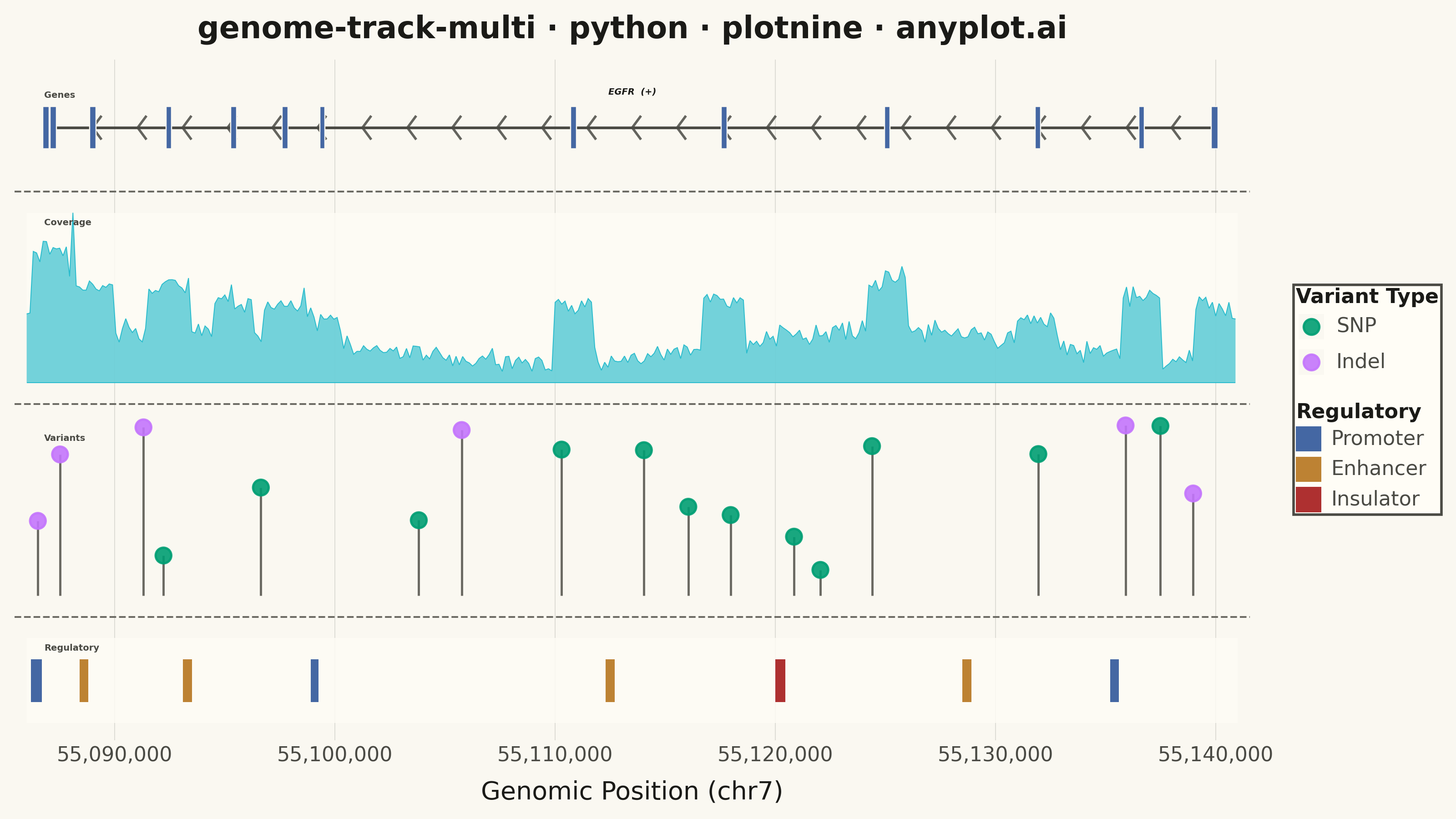
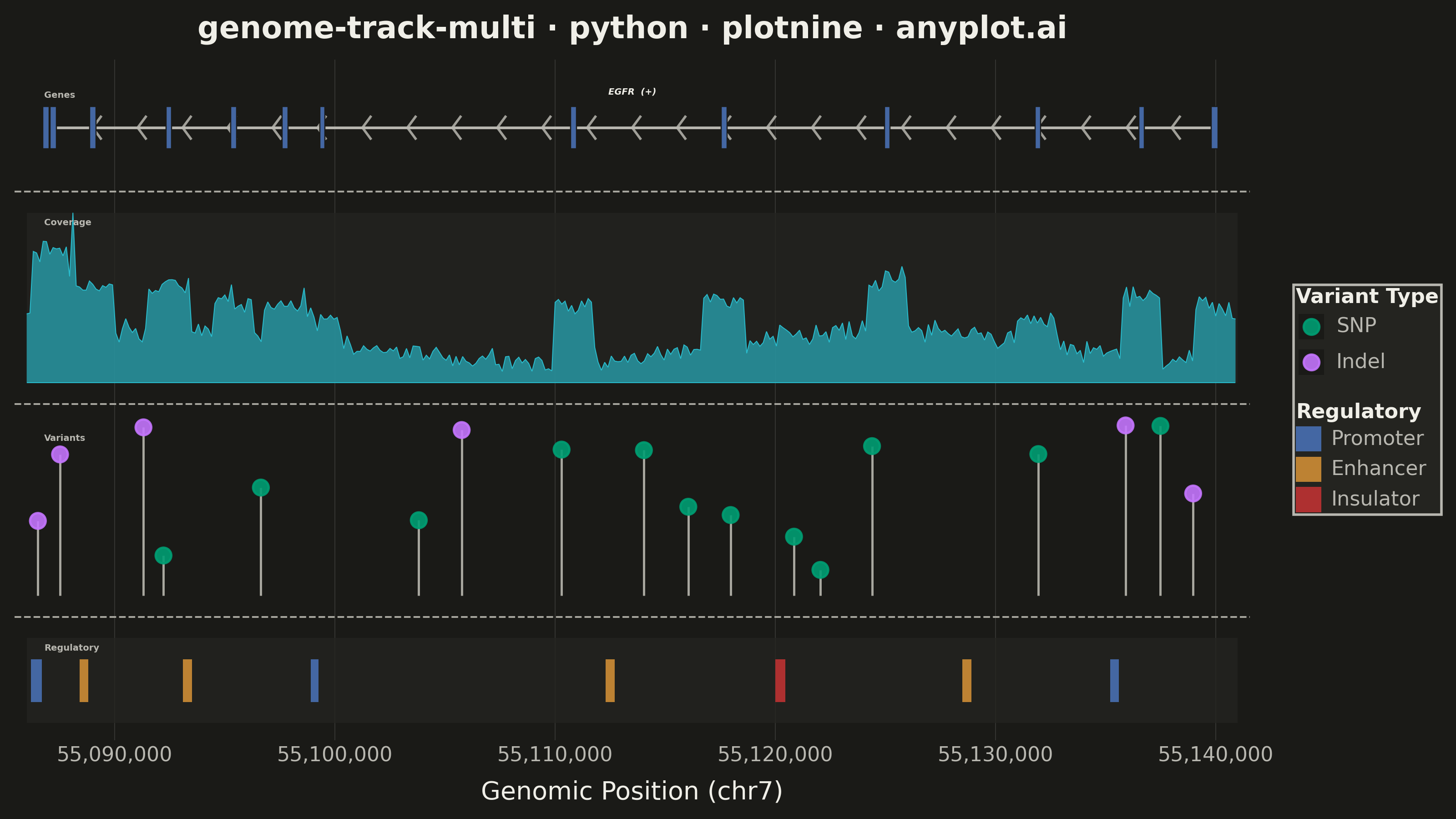
A multi-track genome browser view that displays different types of genomic data aligned along a shared chromosomal coordinate axis. Multiple parallel horizontal tracks (gene annotations, read coverage, variants, regulatory elements) are stacked vertically, each showing a different data type at the same genomic locus. This visualization is essential for integrative genomics, enabling researchers to explore relationships between gene structure, expression, variation, and regulation in a single coordinated view.
""" anyplot.ai
genome-track-multi: Genome Track Viewer
Library: plotnine 0.15.4 | Python 3.13.13
Quality: 89/100 | Updated: 2026-06-02
"""

import os
import sys

import numpy as np
import pandas as pd


# Work around naming conflict with plotnine.py script and plotnine package
_script_dir = os.path.dirname(os.path.abspath(__file__))
for _p in [_script_dir, "", "."]:
    if _p in sys.path:
        sys.path.remove(_p)

from plotnine import (
    aes,
    element_blank,
    element_line,
    element_rect,
    element_text,
    geom_hline,
    geom_point,
    geom_rect,
    geom_ribbon,
    geom_segment,
    geom_text,
    ggplot,
    guide_legend,
    guides,
    labs,
    scale_color_manual,
    scale_fill_manual,
    scale_x_continuous,
    scale_y_continuous,
    theme,
    theme_minimal,
)


np.random.seed(42)

# Theme-adaptive chrome — Imprint palette
THEME = os.getenv("ANYPLOT_THEME", "light")
PAGE_BG = "#FAF8F1" if THEME == "light" else "#1A1A17"
ELEVATED_BG = "#FFFDF6" if THEME == "light" else "#242420"
INK = "#1A1A17" if THEME == "light" else "#F0EFE8"
INK_SOFT = "#4A4A44" if THEME == "light" else "#B8B7B0"
INK_MUTED = "#6B6A63" if THEME == "light" else "#A8A79F"

# Imprint categorical palette — 8 hues, hybrid-v3 sort
IMPRINT = ["#009E73", "#C475FD", "#4467A3", "#BD8233", "#AE3030", "#2ABCCD", "#954477", "#99B314"]

# Genomic region: chr7, EGFR locus (~55kb region)
chrom = "chr7"
region_start = 55_086_000
region_end = 55_141_000

# Track vertical layout (bottom to top):
# Regulatory:  0.0 – 1.0
# Variants:    1.5 – 3.5
# Coverage:    4.0 – 6.0
# Genes:       6.5 – 7.5

# Shaded track backgrounds for regulatory and coverage tracks (theme-adaptive)
track_bg_shaded = pd.DataFrame(
    {"xmin": [region_start, region_start], "xmax": [region_end, region_end], "ymin": [0.0, 4.0], "ymax": [1.0, 6.0]}
)

# Track labels (bold, theme-adaptive ink)
track_labels = pd.DataFrame(
    {
        "x": [region_start + 800] * 4,
        "y": [0.88, 3.35, 5.88, 7.38],
        "label": ["Regulatory", "Variants", "Coverage", "Genes"],
    }
)

# --- Gene Track (center at y=7.0) ---
gene_center = 7.0
exon_half = 0.25

exons = pd.DataFrame(
    {
        "start": [
            55_086_725,
            55_087_058,
            55_088_850,
            55_092_340,
            55_095_262,
            55_097_600,
            55_099_310,
            55_110_700,
            55_117_550,
            55_124_950,
            55_131_800,
            55_136_500,
            55_139_800,
        ],
        "end": [
            55_087_020,
            55_087_350,
            55_089_150,
            55_092_580,
            55_095_530,
            55_097_870,
            55_099_550,
            55_110_960,
            55_117_810,
            55_125_200,
            55_132_050,
            55_136_750,
            55_140_100,
        ],
    }
)
exons["ymin"] = gene_center - exon_half
exons["ymax"] = gene_center + exon_half

intron_lines = pd.DataFrame(
    {
        "x": exons["end"].iloc[:-1].values,
        "xend": exons["start"].iloc[1:].values,
        "y": [gene_center] * (len(exons) - 1),
        "yend": [gene_center] * (len(exons) - 1),
    }
)

# Strand direction chevrons (+ strand) — more prominent than previous iteration
chevron_x = np.linspace(region_start + 3000, region_end - 3000, 25)
chevron_size = 400
chevrons_up = pd.DataFrame(
    {
        "x": chevron_x,
        "xend": chevron_x + chevron_size,
        "y": [gene_center] * len(chevron_x),
        "yend": [gene_center + 0.14] * len(chevron_x),
    }
)
chevrons_down = pd.DataFrame(
    {
        "x": chevron_x,
        "xend": chevron_x + chevron_size,
        "y": [gene_center] * len(chevron_x),
        "yend": [gene_center - 0.14] * len(chevron_x),
    }
)

gene_label = pd.DataFrame({"x": [(region_start + region_end) / 2], "y": [gene_center + 0.42], "label": ["EGFR  (+)"]})

# --- Coverage Track (y: 4.0 – 6.0) ---
cov_base = 4.0
cov_height = 2.0
positions = np.arange(region_start, region_end, 150)
raw_coverage = 25 + 12 * np.sin(np.linspace(0, 3.5 * np.pi, len(positions)))

for _, exon in exons.iterrows():
    mask = (positions >= exon["start"] - 800) & (positions <= exon["end"] + 800)
    raw_coverage[mask] += np.random.uniform(15, 45)

raw_coverage += np.random.normal(0, 4, len(positions))
raw_coverage = np.maximum(raw_coverage, 0)
max_cov = raw_coverage.max()
normalized_cov = raw_coverage / max_cov * cov_height

coverage_df = pd.DataFrame({"x": positions, "ymin": [cov_base] * len(positions), "ymax": cov_base + normalized_cov})

# --- Variant Track (y: 1.5 – 3.5) ---
var_base = 1.5
var_height = 2.0
n_variants = 18
variant_positions = np.sort(np.random.randint(region_start + 500, region_end - 500, n_variants))
variant_quality = np.random.uniform(10, 100, n_variants)
variant_types = np.random.choice(["SNP", "Indel"], n_variants, p=[0.75, 0.25])
normalized_quality = variant_quality / 100.0 * var_height

variant_stems = pd.DataFrame(
    {
        "x": variant_positions,
        "xend": variant_positions,
        "y": [var_base] * n_variants,
        "yend": var_base + normalized_quality,
    }
)

variant_heads = pd.DataFrame(
    {
        "x": variant_positions,
        "y": var_base + normalized_quality,
        "variant_type": pd.Categorical(variant_types, categories=["SNP", "Indel"], ordered=True),
    }
)

# Imprint positions 1→2: SNP (brand green, first series), Indel (lavender — no proximity with ochre Enhancers)
variant_palette = {"SNP": IMPRINT[0], "Indel": IMPRINT[1]}

# --- Regulatory Track (y: 0.0 – 1.0, center at 0.5) ---
reg_center = 0.5
reg_half = 0.25

regulatory_elements = pd.DataFrame(
    {
        "start": [55_086_200, 55_088_400, 55_093_100, 55_098_900, 55_112_300, 55_120_000, 55_128_500, 55_135_200],
        "end": [55_086_700, 55_088_800, 55_093_500, 55_099_250, 55_112_700, 55_120_450, 55_128_900, 55_135_600],
        "feature_type": pd.Categorical(
            ["Promoter", "Enhancer", "Enhancer", "Promoter", "Enhancer", "Insulator", "Enhancer", "Promoter"],
            categories=["Promoter", "Enhancer", "Insulator"],
            ordered=True,
        ),
    }
)
regulatory_elements["ymin"] = reg_center - reg_half
regulatory_elements["ymax"] = reg_center + reg_half

# Imprint positions 3→5: Promoter (blue), Enhancer (ochre), Insulator (red)
regulatory_palette = {"Promoter": IMPRINT[2], "Enhancer": IMPRINT[3], "Insulator": IMPRINT[4]}

# Track separator lines (theme-adaptive dashed)
separators = pd.DataFrame({"yintercept": [1.25, 3.75, 6.25]})

# Build plot with grammar-of-graphics layer composition
plot = (
    ggplot()
    # Shaded track backgrounds (regulatory and coverage tracks)
    + geom_rect(
        data=track_bg_shaded,
        mapping=aes(xmin="xmin", xmax="xmax", ymin="ymin", ymax="ymax"),
        fill=ELEVATED_BG,
        alpha=0.8,
    )
    # Track separators (theme-adaptive)
    + geom_hline(data=separators, mapping=aes(yintercept="yintercept"), color=INK_MUTED, size=0.4, linetype="dashed")
    # Gene track: intron connector lines
    + geom_segment(data=intron_lines, mapping=aes(x="x", xend="xend", y="y", yend="yend"), color=INK_SOFT, size=0.6)
    # Gene track: strand chevrons — increased size and alpha vs previous iteration
    + geom_segment(
        data=chevrons_up, mapping=aes(x="x", xend="xend", y="y", yend="yend"), color=INK_SOFT, size=0.55, alpha=0.85
    )
    + geom_segment(
        data=chevrons_down, mapping=aes(x="x", xend="xend", y="y", yend="yend"), color=INK_SOFT, size=0.55, alpha=0.85
    )
    # Gene track: exon rectangles (Imprint blue)
    + geom_rect(
        data=exons,
        mapping=aes(xmin="start", xmax="end", ymin="ymin", ymax="ymax"),
        fill=IMPRINT[2],
        color=PAGE_BG,
        size=0.25,
    )
    # Gene track: EGFR gene label
    + geom_text(
        data=gene_label,
        mapping=aes(x="x", y="y", label="label"),
        size=3.5,
        color=INK,
        fontstyle="italic",
        fontweight="bold",
    )
    # Coverage track: filled area (Imprint cyan)
    + geom_ribbon(
        data=coverage_df,
        mapping=aes(x="x", ymin="ymin", ymax="ymax"),
        fill=IMPRINT[5],
        alpha=0.65,
        color=IMPRINT[5],
        size=0.2,
    )
    # Variant track: stems (muted structural lines)
    + geom_segment(data=variant_stems, mapping=aes(x="x", xend="xend", y="y", yend="yend"), color=INK_MUTED, size=0.5)
    # Variant track: lollipop heads with Imprint colors (generates native legend)
    + geom_point(data=variant_heads, mapping=aes(x="x", y="y", color="variant_type"), size=3, alpha=0.9)
    + scale_color_manual(name="Variant Type", values=variant_palette, guide=guide_legend(order=1))
    # Regulatory track: colored rectangles with Imprint palette (generates native legend)
    + geom_rect(
        data=regulatory_elements, mapping=aes(xmin="start", xmax="end", ymin="ymin", ymax="ymax", fill="feature_type")
    )
    + scale_fill_manual(name="Regulatory", values=regulatory_palette, guide=guide_legend(order=2))
    # Track labels (theme-adaptive, bold)
    + geom_text(
        data=track_labels,
        mapping=aes(x="x", y="y", label="label"),
        size=3.5,
        ha="left",
        fontweight="bold",
        color=INK_SOFT,
    )
    # Axes
    + scale_x_continuous(
        labels=lambda x: [f"{int(v):,}" for v in x], limits=(region_start, region_end), expand=(0.01, 0)
    )
    + scale_y_continuous(limits=(-0.2, 7.8), breaks=[], expand=(0, 0))
    + labs(title="genome-track-multi · python · plotnine · anyplot.ai", x=f"Genomic Position ({chrom})", y="")
    # Theme-adaptive chrome (Imprint palette canonical tokens)
    + theme_minimal()
    + theme(
        figure_size=(8, 4.5),
        plot_title=element_text(size=12, weight="bold", color=INK),
        axis_title_x=element_text(size=10, color=INK),
        axis_title_y=element_blank(),
        axis_text_x=element_text(size=8, color=INK_SOFT),
        axis_text_y=element_blank(),
        axis_ticks_major_y=element_blank(),
        legend_title=element_text(size=8, weight="bold", color=INK),
        legend_text=element_text(size=8, color=INK_SOFT),
        legend_position="right",
        legend_background=element_rect(fill=ELEVATED_BG, color=INK_SOFT),
        legend_key_size=10,
        panel_grid_minor=element_blank(),
        panel_grid_major_x=element_line(color=INK, size=0.3, alpha=0.15),
        panel_grid_major_y=element_blank(),
        panel_background=element_rect(fill=PAGE_BG, color=None),
        plot_background=element_rect(fill=PAGE_BG, color=PAGE_BG),
    )
    + guides(fill=guide_legend(override_aes={"alpha": 1}))
)

# Save — landscape 3200×1800 px (8 in × 4.5 in @ 400 dpi)
plot.save(f"plot-{THEME}.png", dpi=400, width=8, height=4.5, units="in")
Runnable source as JSON, for any HTTP client: https://api.anyplot.ai/specs/genome-track-multi/plotnine/code. Any spec id and library id listed in llms-full.txt fit the same URL shape; every URL below is complete and callable.
{
  "spec_id": "genome-track-multi",
  "language": "python",
  "library": "plotnine",
  "page": "https://anyplot.ai/genome-track-multi/python/plotnine",
  "hub": "https://anyplot.ai/genome-track-multi",
  "code_json": "https://api.anyplot.ai/specs/genome-track-multi/plotnine/code",
  "spec_json": "https://api.anyplot.ai/specs/genome-track-multi",
  "render_light_png": "https://storage.googleapis.com/anyplot-images/plots/genome-track-multi/python/plotnine/plot-light.png",
  "render_dark_png": "https://storage.googleapis.com/anyplot-images/plots/genome-track-multi/python/plotnine/plot-dark.png",
  "quality_score": 89.0,
  "license": "MIT",
  "guide": "https://anyplot.ai/llms.txt"
}
Part of Genome Track Viewer on anyplot.ai.