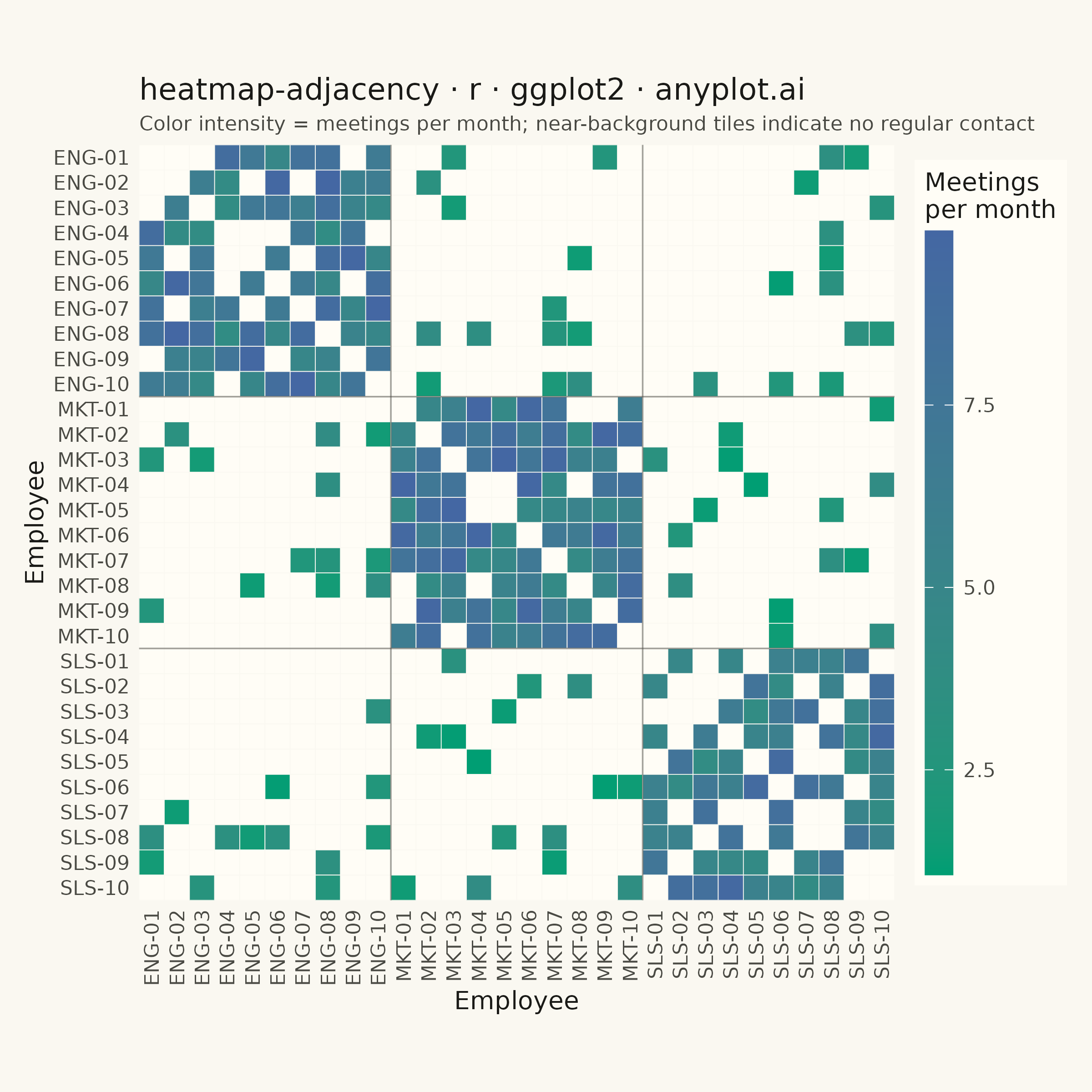
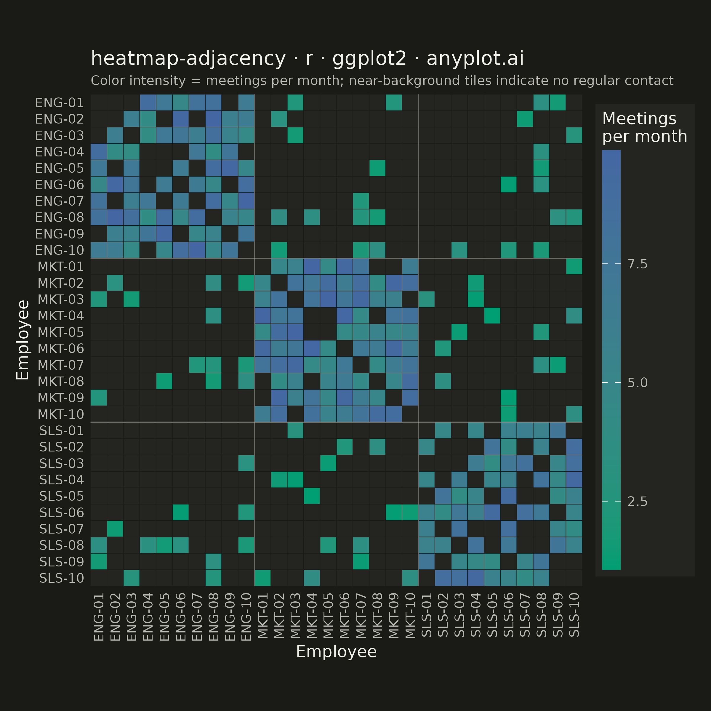
The same plot in 14 other libraries — Python: Altair, Bokeh, lets-plot, Matplotlib, Plotly, plotnine, Pygal, Seaborn; Julia: Makie.jl; JavaScript: Chart.js, D3.js, Apache ECharts, Highcharts, MUI X Charts. Compare all 15 side by side: Network Adjacency Matrix Heatmap in Python, R, Julia and JavaScript.
A matrix-based representation of a network or graph where rows and columns represent nodes and cell color indicates the presence or weight of edges between them. This visualization complements node-link diagrams by excelling at revealing clusters, structural patterns, and density in large or dense networks where node-link layouts become cluttered. Reordering nodes by cluster, degree, or community membership exposes block-diagonal structure and makes group boundaries immediately visible.
#' anyplot.ai
#' heatmap-adjacency: Network Adjacency Matrix Heatmap
#' Library: ggplot2 3.5.1 | R 4.4.1
#' Quality: 92/100 | Created: 2026-09-05

library(ggplot2)
library(dplyr)
library(tidyr)
library(ragg)

set.seed(42)

# --- Theme tokens ------------------------------------------------------------
THEME       <- Sys.getenv("ANYPLOT_THEME", "light")
PAGE_BG     <- if (THEME == "light") "#FAF8F1" else "#1A1A17"
ELEVATED_BG <- if (THEME == "light") "#FFFDF6" else "#242420"
INK         <- if (THEME == "light") "#1A1A17" else "#F0EFE8"
INK_SOFT    <- if (THEME == "light") "#4A4A44" else "#B8B7B0"

# --- Data: coworker collaboration network ------------------------------------
# 30 employees across 3 departments; node labels carry the department prefix
# so group boundaries are visible directly in the axis ticks (per spec note
# on large networks). Within-department pairs collaborate more often and more
# intensely than cross-department pairs, producing block-diagonal structure.
departments <- c("Engineering", "Marketing", "Sales")
dept_short  <- c(Engineering = "ENG", Marketing = "MKT", Sales = "SLS")
n_per_dept  <- 10

nodes <- tibble::tibble(department = rep(departments, each = n_per_dept)) %>%
  group_by(department) %>%
  mutate(idx = row_number()) %>%
  ungroup() %>%
  mutate(node = sprintf("%s-%02d", dept_short[department], idx))

n_nodes <- nrow(nodes)

weight_mat <- matrix(NA_real_, n_nodes, n_nodes)
for (i in seq_len(n_nodes)) {
  for (j in seq_len(n_nodes)) {
    if (j <= i) next
    same_dept <- nodes$department[i] == nodes$department[j]
    edge_prob <- if (same_dept) 0.75 else 0.12
    if (runif(1) < edge_prob) {
      weight <- if (same_dept) runif(1, 4, 10) else runif(1, 1, 4)
      weight_mat[i, j] <- weight
      weight_mat[j, i] <- weight # undirected graph: fill both triangles
    }
  }
}
rownames(weight_mat) <- nodes$node
colnames(weight_mat) <- nodes$node

adjacency_df <- as.data.frame(weight_mat) %>%
  tibble::rownames_to_column("source") %>%
  pivot_longer(-source, names_to = "target", values_to = "weight") %>%
  mutate(
    source = factor(source, levels = nodes$node),
    target = factor(target, levels = nodes$node)
  )

# --- Department-boundary markers ---------------------------------------
# Positions along each discrete axis where one department's block ends and
# the next begins, drawn as subtle divider lines to reinforce the
# block-diagonal structure beyond what tick labels alone convey.
boundaries <- head(cumsum(table(nodes$department)[departments]), -1) + 0.5

# --- Plot ---------------------------------------------------------------
p <- ggplot(adjacency_df, aes(x = target, y = source, fill = weight)) +
  geom_tile(color = PAGE_BG, linewidth = 0.15) +
  geom_vline(xintercept = boundaries, color = INK_SOFT, linewidth = 0.3, alpha = 0.5) +
  geom_hline(yintercept = boundaries, color = INK_SOFT, linewidth = 0.3, alpha = 0.5) +
  scale_fill_gradient(
    low      = "#009E73",
    high     = "#4467A3",
    na.value = ELEVATED_BG, # absent edges (incl. diagonal): near-bg, distinct from data
    name     = "Meetings\nper month",
    guide    = guide_colorbar(barheight = unit(9, "cm"), barwidth = unit(0.4, "cm"))
  ) +
  scale_x_discrete(expand = c(0, 0)) +
  scale_y_discrete(expand = c(0, 0), limits = rev(nodes$node)) +
  coord_fixed(ratio = 1) +
  labs(
    title    = "heatmap-adjacency · r · ggplot2 · anyplot.ai",
    subtitle = "Color intensity = meetings per month; near-background tiles indicate no regular contact",
    x = "Employee", y = "Employee"
  ) +
  theme_minimal(base_size = 8) +
  theme(
    plot.background    = element_rect(fill = PAGE_BG, color = PAGE_BG),
    panel.background   = element_rect(fill = PAGE_BG, color = NA),
    panel.grid         = element_blank(),
    axis.title         = element_text(color = INK, size = 10),
    axis.text.x        = element_text(color = INK_SOFT, size = 8, angle = 90, hjust = 1, vjust = 0.5),
    axis.text.y        = element_text(color = INK_SOFT, size = 8),
    plot.title         = element_text(color = INK, size = 12),
    plot.subtitle      = element_text(color = INK_SOFT, size = 8),
    legend.text        = element_text(color = INK_SOFT, size = 8),
    legend.title       = element_text(color = INK, size = 10),
    legend.background  = element_rect(fill = ELEVATED_BG, color = NA),
    plot.margin        = margin(10, 10, 10, 10)
  )

# --- Save ---------------------------------------------------------------
ggsave(
  filename = sprintf("plot-%s.png", THEME),
  plot     = p,
  device   = ragg::agg_png,
  width    = 6,
  height   = 6,
  units    = "in",
  dpi      = 400
)
Runnable source as JSON, for any HTTP client: https://api.anyplot.ai/specs/heatmap-adjacency/ggplot2/code. Any spec id and library id listed in llms-full.txt fit the same URL shape; every URL below is complete and callable.
{
  "spec_id": "heatmap-adjacency",
  "language": "r",
  "library": "ggplot2",
  "page": "https://anyplot.ai/heatmap-adjacency/r/ggplot2",
  "hub": "https://anyplot.ai/heatmap-adjacency",
  "code_json": "https://api.anyplot.ai/specs/heatmap-adjacency/ggplot2/code",
  "spec_json": "https://api.anyplot.ai/specs/heatmap-adjacency",
  "render_light_png": "https://storage.googleapis.com/anyplot-images/plots/heatmap-adjacency/r/ggplot2/plot-light.png",
  "render_dark_png": "https://storage.googleapis.com/anyplot-images/plots/heatmap-adjacency/r/ggplot2/plot-dark.png",
  "quality_score": 92.0,
  "license": "MIT",
  "guide": "https://anyplot.ai/llms.txt"
}
Part of Network Adjacency Matrix Heatmap on anyplot.ai.