The same plot in 14 other libraries — Python: Altair, Bokeh, lets-plot, Matplotlib, Plotly, plotnine, Pygal, Seaborn; Julia: Makie.jl; JavaScript: Chart.js, D3.js, Apache ECharts, Highcharts, MUI X Charts. Compare all 15 side by side: Clustered Heatmap in Python, R, Julia and JavaScript.
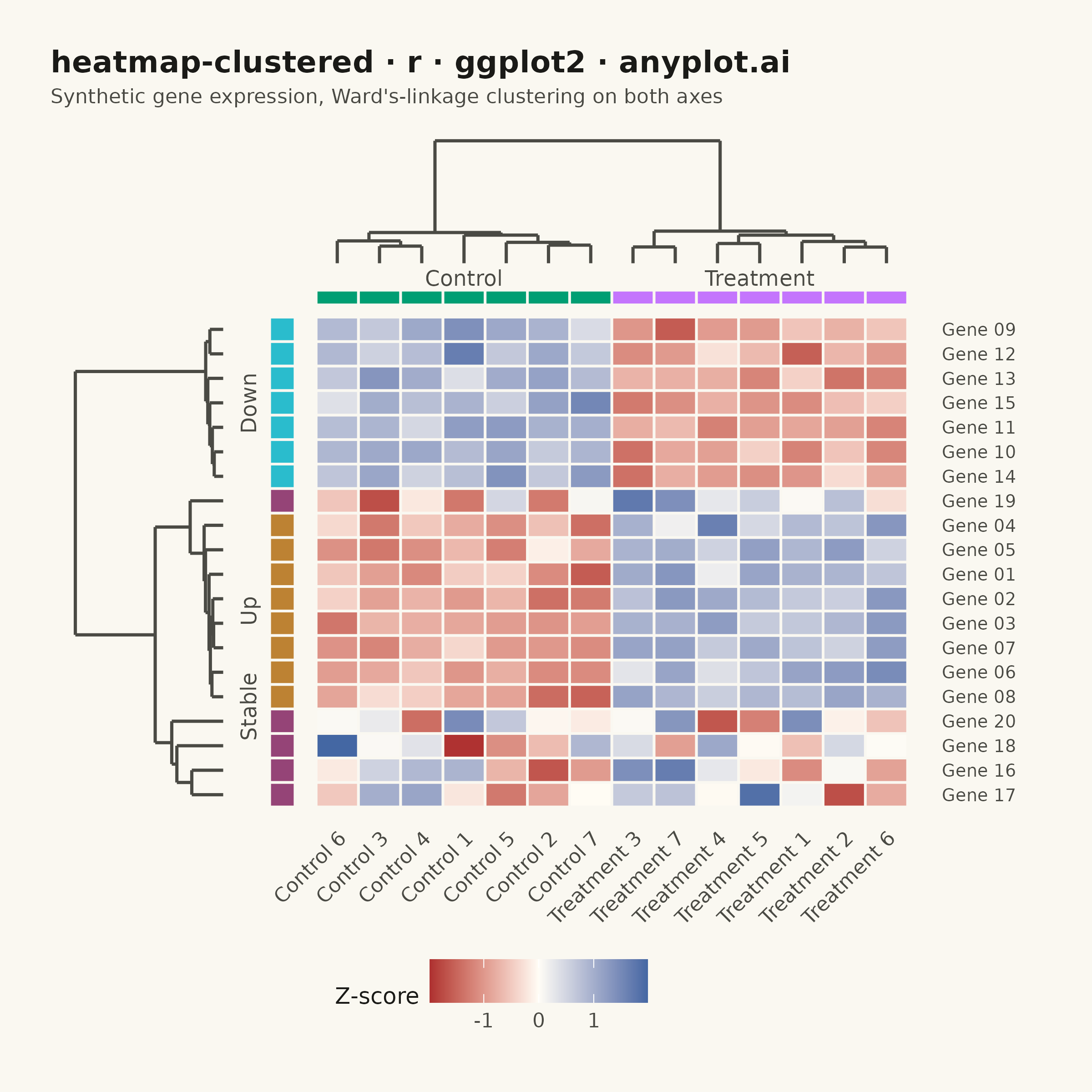
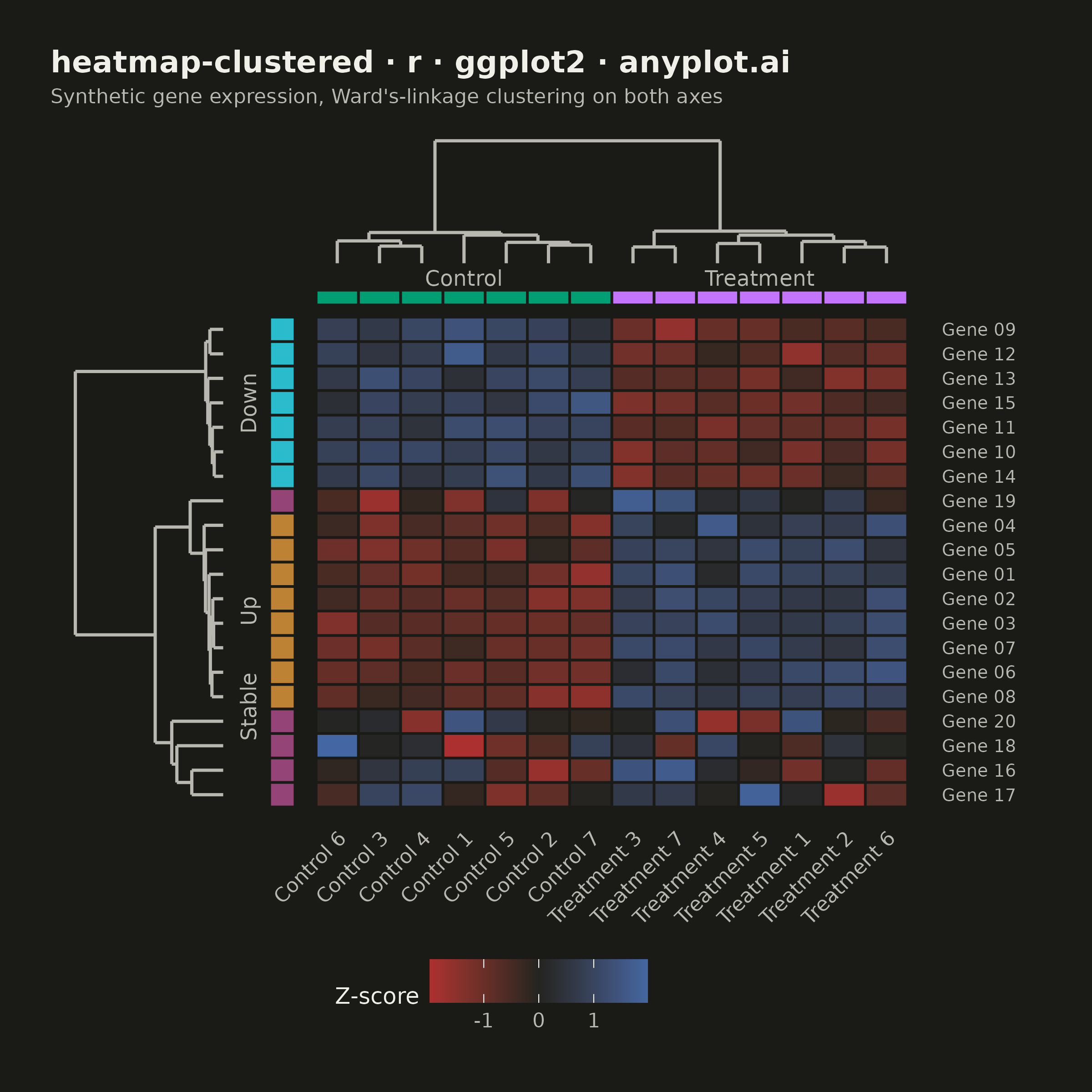
A heatmap with hierarchical clustering dendrograms on both rows and columns, showing both data values and their hierarchical relationships. Rows and columns are automatically reordered based on clustering results to reveal natural groupings in the data. Essential for discovering patterns in high-dimensional data where similar observations or variables should be visually grouped together.
#' anyplot.ai
#' heatmap-clustered: Clustered Heatmap
#' Library: ggplot2 3.5.1 | R 4.4.1
#' Quality: 96/100 | Created: 2026-09-05

library(ggplot2)
library(ragg)

set.seed(42)

# --- Theme tokens ------------------------------------------------------------
THEME       <- Sys.getenv("ANYPLOT_THEME", "light")
PAGE_BG     <- if (THEME == "light") "#FAF8F1" else "#1A1A17"
ELEVATED_BG <- if (THEME == "light") "#FFFDF6" else "#242420"
INK         <- if (THEME == "light") "#1A1A17" else "#F0EFE8"
INK_SOFT    <- if (THEME == "light") "#4A4A44" else "#B8B7B0"
# Distinct from PAGE_BG (not equal) so near-zero z-score tiles stay visible
# as part of the grid instead of fading into the canvas.
DIV_MID     <- ELEVATED_BG
IMPRINT_PALETTE <- c("#009E73", "#C475FD", "#4467A3", "#BD8233",
                     "#AE3030", "#2ABCCD", "#954477", "#99B314")

# --- Data: synthetic gene-expression matrix ----------------------------------
# 20 genes across 14 samples (7 control, 7 treatment); three latent gene
# programs create block structure for clustering to recover.
n_genes   <- 20
n_samples <- 14
gene_module  <- rep(c("Up", "Down", "Stable"), c(8, 7, 5))
sample_group <- rep(c("Control", "Treatment"), each = 7)
gene_id      <- sprintf("Gene %02d", seq_len(n_genes))
sample_id    <- c(paste("Control", 1:7), paste("Treatment", 1:7))

expr <- matrix(rnorm(n_genes * n_samples, mean = 0, sd = 0.45),
               nrow = n_genes, ncol = n_samples,
               dimnames = list(gene_id, sample_id))
treat_cols <- sample_group == "Treatment"
expr[gene_module == "Up",   treat_cols] <- expr[gene_module == "Up",   treat_cols] + 2.3
expr[gene_module == "Down", treat_cols] <- expr[gene_module == "Down", treat_cols] - 2.3

# Per-gene z-score so every row is centered before clustering & coloring
expr_z <- t(scale(t(expr)))

# --- Hierarchical clustering (Ward's linkage) --------------------------------
row_hc <- hclust(dist(expr_z), method = "ward.D2")
col_hc <- hclust(dist(t(expr_z)), method = "ward.D2")

# Heatmap coordinates: leaf order sets 1..n grid position along each axis.
# Rows are flipped so the first leaf in clustering order sits at the top.
row_rank <- integer(n_genes)
row_rank[row_hc$order] <- seq_len(n_genes)
row_leaf_y <- n_genes - row_rank + 1

col_rank <- integer(n_samples)
col_rank[col_hc$order] <- seq_len(n_samples)
col_leaf_x <- col_rank

# --- Heatmap tile data --------------------------------------------------------
tile_df <- expand.grid(gene_i = seq_len(n_genes), sample_j = seq_len(n_samples))
tile_df$value  <- expr_z[cbind(tile_df$gene_i, tile_df$sample_j)]
tile_df$x      <- col_leaf_x[tile_df$sample_j]
tile_df$y      <- row_leaf_y[tile_df$gene_i]

x_axis_labels <- sample_id[col_hc$order]
y_axis_labels <- gene_id[rev(row_hc$order)]

# --- Row group annotation strip (gene module) --------------------------------
ROW_ANN_THICK <- 0.6
ROW_ANN_X     <- -0.3
row_color_map <- c(Up = IMPRINT_PALETTE[4], Down = IMPRINT_PALETTE[6], Stable = IMPRINT_PALETTE[7])
row_ann_df <- data.frame(
  y     = row_leaf_y,
  group = gene_module,
  color = row_color_map[gene_module]
)
row_ann_label_df <- data.frame(
  y     = tapply(row_ann_df$y, row_ann_df$group, mean),
  label = names(tapply(row_ann_df$y, row_ann_df$group, mean))
)
ROW_LABEL_X <- ROW_ANN_X - ROW_ANN_THICK / 2 - 0.5

# --- Row dendrogram: rotated (height -> x, leaf position -> y) ---------------
# Placed left of the row annotation strip; leaves touch ROW_LEAF_X, root extends left.
ROW_LEAF_X     <- ROW_LABEL_X - 0.6
row_dend_width <- 3.5
row_h_scale    <- row_dend_width / max(row_hc$height)

n_row_merges <- n_genes - 1
row_node_y   <- numeric(n_row_merges)
for (k in seq_len(n_row_merges)) {
  lft <- row_hc$merge[k, 1]
  rgt <- row_hc$merge[k, 2]
  yl  <- if (lft < 0) row_leaf_y[-lft] else row_node_y[lft]
  yr  <- if (rgt < 0) row_leaf_y[-rgt] else row_node_y[rgt]
  row_node_y[k] <- (yl + yr) / 2
}

n_row_segs  <- 3L * n_row_merges
row_seg_h    <- numeric(n_row_segs)
row_seg_hend <- numeric(n_row_segs)
row_seg_y    <- numeric(n_row_segs)
row_seg_yend <- numeric(n_row_segs)
for (k in seq_len(n_row_merges)) {
  lft <- row_hc$merge[k, 1]
  rgt <- row_hc$merge[k, 2]
  yl  <- if (lft < 0) row_leaf_y[-lft] else row_node_y[lft]
  hl  <- if (lft < 0) 0                else row_hc$height[lft]
  yr  <- if (rgt < 0) row_leaf_y[-rgt] else row_node_y[rgt]
  hr  <- if (rgt < 0) 0                else row_hc$height[rgt]
  Hk  <- row_hc$height[k]
  i <- (k - 1L) * 3L + 1L
  row_seg_h[i]      <- hl; row_seg_hend[i]      <- Hk; row_seg_y[i]      <- yl; row_seg_yend[i]      <- yl
  row_seg_h[i + 1L] <- Hk; row_seg_hend[i + 1L] <- Hk; row_seg_y[i + 1L] <- yl; row_seg_yend[i + 1L] <- yr
  row_seg_h[i + 2L] <- hr; row_seg_hend[i + 2L] <- Hk; row_seg_y[i + 2L] <- yr; row_seg_yend[i + 2L] <- yr
}
row_dend_df <- data.frame(
  x    = ROW_LEAF_X - row_seg_h * row_h_scale,
  xend = ROW_LEAF_X - row_seg_hend * row_h_scale,
  y    = row_seg_y,
  yend = row_seg_yend
)

# --- Column group annotation strip (Control / Treatment) --------------------
ANN_Y      <- n_genes + 0.5 + 0.5 + 0.3
ANN_THICK  <- 0.6
ann_df <- data.frame(
  x     = col_leaf_x,
  group = sample_group,
  color = ifelse(sample_group == "Control", IMPRINT_PALETTE[1], IMPRINT_PALETTE[2])
)
ann_label_df <- data.frame(
  x     = tapply(ann_df$x, ann_df$group, mean),
  label = names(tapply(ann_df$x, ann_df$group, mean))
)

# --- Column dendrogram: standard orientation (leaf position -> x, height -> y)
COL_LEAF_Y     <- ANN_Y + ANN_THICK / 2 + 1.1
col_dend_height <- 5
col_h_scale     <- col_dend_height / max(col_hc$height)

n_col_merges <- n_samples - 1
col_node_x   <- numeric(n_col_merges)
for (k in seq_len(n_col_merges)) {
  lft <- col_hc$merge[k, 1]
  rgt <- col_hc$merge[k, 2]
  xl  <- if (lft < 0) col_leaf_x[-lft] else col_node_x[lft]
  xr  <- if (rgt < 0) col_leaf_x[-rgt] else col_node_x[rgt]
  col_node_x[k] <- (xl + xr) / 2
}

n_col_segs   <- 3L * n_col_merges
col_seg_x    <- numeric(n_col_segs)
col_seg_xend <- numeric(n_col_segs)
col_seg_h    <- numeric(n_col_segs)
col_seg_hend <- numeric(n_col_segs)
for (k in seq_len(n_col_merges)) {
  lft <- col_hc$merge[k, 1]
  rgt <- col_hc$merge[k, 2]
  xl  <- if (lft < 0) col_leaf_x[-lft] else col_node_x[lft]
  hl  <- if (lft < 0) 0                else col_hc$height[lft]
  xr  <- if (rgt < 0) col_leaf_x[-rgt] else col_node_x[rgt]
  hr  <- if (rgt < 0) 0                else col_hc$height[rgt]
  Hk  <- col_hc$height[k]
  i <- (k - 1L) * 3L + 1L
  col_seg_x[i]      <- xl; col_seg_xend[i]      <- xl; col_seg_h[i]      <- hl; col_seg_hend[i]      <- Hk
  col_seg_x[i + 1L] <- xl; col_seg_xend[i + 1L] <- xr; col_seg_h[i + 1L] <- Hk; col_seg_hend[i + 1L] <- Hk
  col_seg_x[i + 2L] <- xr; col_seg_xend[i + 2L] <- xr; col_seg_h[i + 2L] <- hr; col_seg_hend[i + 2L] <- Hk
}
col_dend_df <- data.frame(
  x    = col_seg_x,
  xend = col_seg_xend,
  y    = COL_LEAF_Y + col_seg_h * col_h_scale,
  yend = COL_LEAF_Y + col_seg_hend * col_h_scale
)

max_abs <- max(abs(range(expr_z)))
plot_title    <- "heatmap-clustered · r · ggplot2 · anyplot.ai"
plot_subtitle <- "Synthetic gene expression, Ward's-linkage clustering on both axes"

# --- Plot ---------------------------------------------------------------------
p <- ggplot() +
  geom_tile(
    data = tile_df, aes(x = x, y = y, fill = value),
    color = PAGE_BG, linewidth = 0.5
  ) +
  geom_tile(
    data = ann_df, aes(x = x, y = ANN_Y, fill = I(color)),
    color = PAGE_BG, linewidth = 0.5, height = ANN_THICK
  ) +
  geom_text(
    data = ann_label_df, aes(x = x, y = ANN_Y + ANN_THICK / 2 + 0.5, label = label),
    color = INK_SOFT, size = 3.0
  ) +
  geom_tile(
    data = row_ann_df, aes(x = ROW_ANN_X, y = y, fill = I(color)),
    color = PAGE_BG, linewidth = 0.5, width = ROW_ANN_THICK
  ) +
  geom_text(
    data = row_ann_label_df, aes(x = ROW_LABEL_X, y = y, label = label),
    color = INK_SOFT, size = 3.0, angle = 90
  ) +
  geom_segment(
    data = row_dend_df, aes(x = x, xend = xend, y = y, yend = yend),
    color = INK_SOFT, linewidth = 0.6
  ) +
  geom_segment(
    data = col_dend_df, aes(x = x, xend = xend, y = y, yend = yend),
    color = INK_SOFT, linewidth = 0.6
  ) +
  scale_fill_gradient2(
    low = "#AE3030", mid = DIV_MID, high = "#4467A3",
    midpoint = 0, limits = c(-max_abs, max_abs), name = "Z-score"
  ) +
  scale_x_continuous(breaks = seq_len(n_samples), labels = x_axis_labels,
                     expand = expansion(mult = 0.03)) +
  scale_y_continuous(breaks = seq_len(n_genes), labels = y_axis_labels,
                     position = "right", expand = expansion(mult = 0.02)) +
  labs(title = plot_title, subtitle = plot_subtitle, x = NULL, y = NULL) +
  theme_minimal(base_size = 8) +
  theme(
    plot.background   = element_rect(fill = PAGE_BG, color = PAGE_BG),
    panel.background  = element_rect(fill = PAGE_BG, color = NA),
    panel.grid        = element_blank(),
    axis.ticks        = element_blank(),
    axis.text.x       = element_text(color = INK_SOFT, size = 8, angle = 45, hjust = 1),
    axis.text.y       = element_text(color = INK_SOFT, size = 7),
    plot.title        = element_text(color = INK, size = 12, face = "bold",
                                     margin = margin(b = 4)),
    plot.subtitle     = element_text(color = INK_SOFT, size = 8,
                                     margin = margin(b = 8)),
    legend.background = element_rect(fill = NA, color = NA),
    legend.text       = element_text(color = INK_SOFT, size = 8),
    legend.title      = element_text(color = INK, size = 9),
    legend.position   = "bottom",
    plot.margin       = margin(20, 30, 20, 20)
  )

# --- Save (square canvas: 2400x2400 px = 6in x 6in @ 400 dpi) ---------------
ggsave(
  filename = sprintf("plot-%s.png", THEME),
  plot     = p,
  device   = ragg::agg_png,
  width    = 6,
  height   = 6,
  units    = "in",
  dpi      = 400
)
Runnable source as JSON, for any HTTP client: https://api.anyplot.ai/specs/heatmap-clustered/ggplot2/code. Any spec id and library id listed in llms-full.txt fit the same URL shape; every URL below is complete and callable.
{
  "spec_id": "heatmap-clustered",
  "language": "r",
  "library": "ggplot2",
  "page": "https://anyplot.ai/heatmap-clustered/r/ggplot2",
  "hub": "https://anyplot.ai/heatmap-clustered",
  "code_json": "https://api.anyplot.ai/specs/heatmap-clustered/ggplot2/code",
  "spec_json": "https://api.anyplot.ai/specs/heatmap-clustered",
  "render_light_png": "https://storage.googleapis.com/anyplot-images/plots/heatmap-clustered/r/ggplot2/plot-light.png",
  "render_dark_png": "https://storage.googleapis.com/anyplot-images/plots/heatmap-clustered/r/ggplot2/plot-dark.png",
  "quality_score": 96.0,
  "license": "MIT",
  "guide": "https://anyplot.ai/llms.txt"
}
Part of Clustered Heatmap on anyplot.ai.