The same plot in 14 other libraries — JavaScript: Chart.js, Apache ECharts, Highcharts, MUI X Charts; Python: Altair, Bokeh, lets-plot, Matplotlib, Plotly, plotnine, Pygal, Seaborn; R: ggplot2; Julia: Makie.jl. Compare all 15 side by side: Rainflow Counting Matrix for Fatigue Analysis in Python, R, Julia and JavaScript.
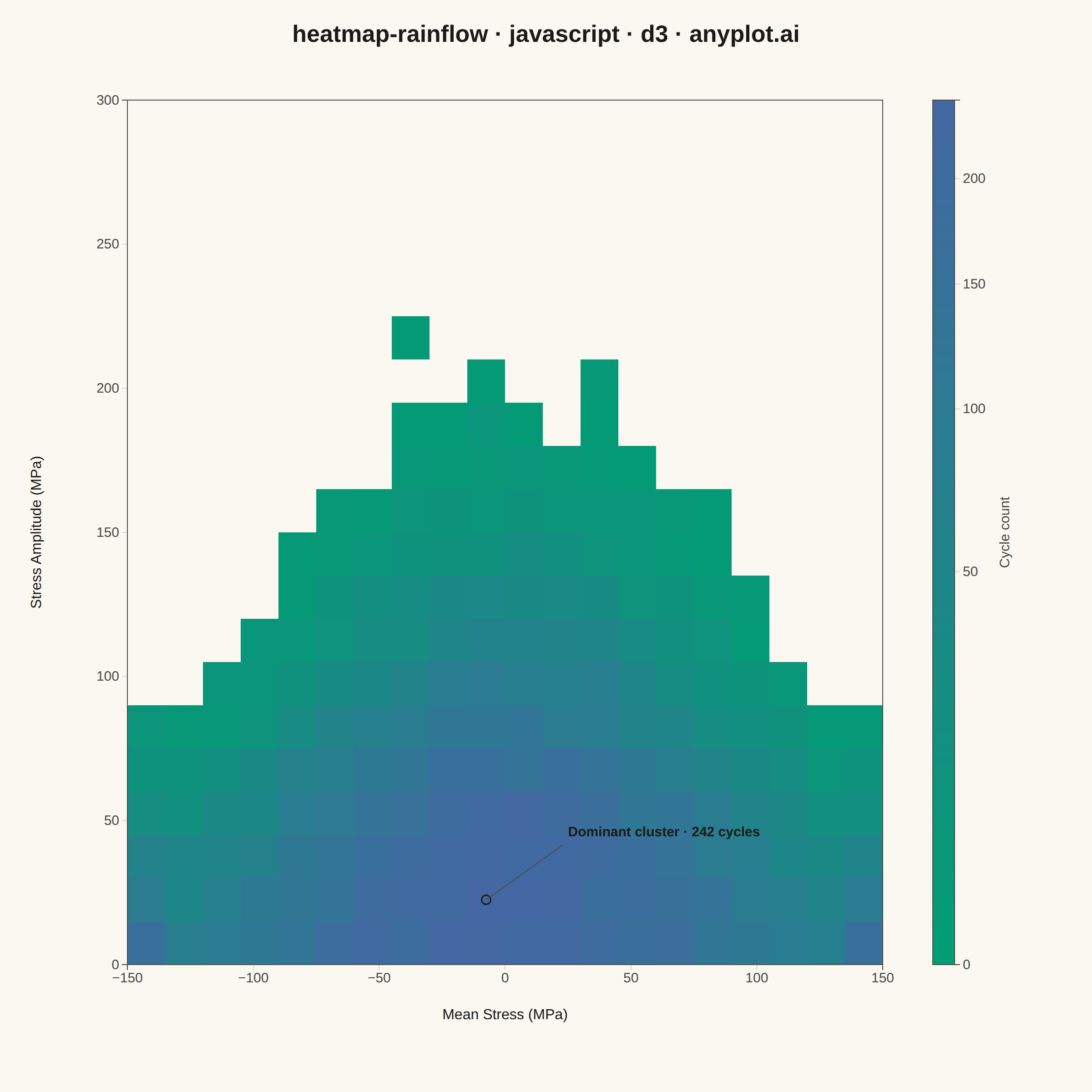
A rainflow counting matrix visualizes the results of rainflow cycle counting from a load or stress time history. The matrix displays cycle counts as a 2D heatmap where one axis represents cycle amplitude (half-range), the other represents cycle mean value, and color intensity represents the frequency of each cycle combination. This is a fundamental tool in fatigue analysis and durability engineering, used to characterize variable-amplitude loading for fatigue life prediction.
// anyplot.ai
// heatmap-rainflow: Rainflow Counting Matrix for Fatigue Analysis
// Library: d3 7.9.0 | JavaScript 22.23.2
// Quality: 89/100 | Created: 2026-08-25

//# anyplot-orientation: square
const t = window.ANYPLOT_TOKENS;
const { width, height } = window.ANYPLOT_SIZE;

// --- Deterministic PRNG (LCG) + Box-Muller normal sampler --------------------
// The browser has no seeded RNG, so a tiny linear-congruential generator
// stands in for numpy's `seed(42)` — same role, reproducible cycle counts.
let lcgState = 42;
function rand() {
  lcgState = (1664525 * lcgState + 1013904223) >>> 0;
  return lcgState / 4294967296;
}
function normal() {
  const u1 = Math.max(rand(), 1e-12);
  const u2 = rand();
  return Math.sqrt(-2 * Math.log(u1)) * Math.cos(2 * Math.PI * u2);
}

// --- Synthetic load history -> binned rainflow matrix ------------------------
// Simulates the output of rainflow cycle counting on a variable-amplitude
// stress history: many small, widely-scattered cycles and a tapering tail of
// rare large-amplitude cycles that cluster near zero mean stress — the classic
// "teardrop" envelope seen in measured fatigue load spectra.
const ampMax = 300; // MPa, half-range
const meanMin = -150;
const meanMax = 150; // MPa
const ampBins = 20;
const meanBins = 20;
const ampStep = ampMax / ampBins;
const meanStep = (meanMax - meanMin) / meanBins;
const cycleCount = 15000;

const matrix = Array.from({ length: ampBins }, () => new Array(meanBins).fill(0));
for (let i = 0; i < cycleCount; i++) {
  const amplitude = Math.min(ampMax - 1e-6, Math.abs(normal()) * 55);
  const meanSigma = 20 + 70 * Math.exp(-amplitude / 90);
  const mean = Math.min(meanMax - 1e-6, Math.max(meanMin, normal() * meanSigma));

  const ai = Math.min(ampBins - 1, Math.floor(amplitude / ampStep));
  const mi = Math.min(meanBins - 1, Math.max(0, Math.floor((mean - meanMin) / meanStep)));
  matrix[ai][mi]++;
}

const cells = [];
for (let ai = 0; ai < ampBins; ai++) {
  for (let mi = 0; mi < meanBins; mi++) {
    cells.push({
      ampLo: ai * ampStep,
      ampHi: (ai + 1) * ampStep,
      meanLo: meanMin + mi * meanStep,
      meanHi: meanMin + (mi + 1) * meanStep,
      count: matrix[ai][mi],
    });
  }
}
const maxCount = d3.max(cells, (d) => d.count);

// --- Layout -------------------------------------------------------------------
const margin = { top: 110, right: 230, bottom: 140, left: 140 };
const iw = width - margin.left - margin.right;
const ih = height - margin.top - margin.bottom;

const svg = d3.select("#container").append("svg").attr("width", width).attr("height", height);
const g = svg.append("g").attr("transform", `translate(${margin.left},${margin.top})`);

// --- Scales -------------------------------------------------------------------
const x = d3.scaleLinear().domain([meanMin, meanMax]).range([0, iw]);
const y = d3.scaleLinear().domain([0, ampMax]).range([ih, 0]);

// Cycle counts are single-polarity (non-negative), so the Imprint sequential
// ramp applies. A sqrt transform spreads the many low-count bins across more
// of the ramp instead of leaving them a flat near-uniform green.
const colorPos = d3.scaleSqrt().domain([0, maxCount]).range([0, 1]).clamp(true);
const cellColor = (count) => d3.interpolateRgbBasis(t.seq)(colorPos(count));

// --- Matrix cells ---------------------------------------------------------
// No per-cell stroke: at 20x20 resolution a uniform grid of strokes plus the
// outer frame reads busy. The outer frame alone is enough to enclose the grid.
g.selectAll("rect.cell")
  .data(cells)
  .join("rect")
  .attr("class", "cell")
  .attr("x", (d) => x(d.meanLo))
  .attr("y", (d) => y(d.ampHi))
  .attr("width", (d) => x(d.meanHi) - x(d.meanLo))
  .attr("height", (d) => y(d.ampLo) - y(d.ampHi))
  .attr("fill", (d) => (d.count > 0 ? cellColor(d.count) : t.pageBg));

g.append("rect")
  .attr("x", 0)
  .attr("y", 0)
  .attr("width", iw)
  .attr("height", ih)
  .attr("fill", "none")
  .attr("stroke", t.inkSoft)
  .attr("stroke-width", 1);

// --- Dominant-cluster callout -----------------------------------------------
// Gives the highest-count bin an explicit focal point, directly supporting the
// spec's "identifying dominant cycle combinations" fatigue-analysis use case.
const peakCell = cells.reduce((best, d) => (d.count > best.count ? d : best), cells[0]);
const peakX = x((peakCell.meanLo + peakCell.meanHi) / 2);
const peakY = y((peakCell.ampLo + peakCell.ampHi) / 2);
const calloutX = Math.min(peakX + 90, iw - 210);
const calloutY = Math.max(peakY - 70, 28);

g.append("circle")
  .attr("cx", peakX)
  .attr("cy", peakY)
  .attr("r", 5)
  .attr("fill", "none")
  .attr("stroke", t.ink)
  .attr("stroke-width", 1.5);

g.append("line")
  .attr("x1", peakX)
  .attr("y1", peakY)
  .attr("x2", calloutX - 6)
  .attr("y2", calloutY + 10)
  .attr("stroke", t.inkSoft)
  .attr("stroke-width", 1);

g.append("text")
  .attr("x", calloutX)
  .attr("y", calloutY)
  .attr("text-anchor", "start")
  .attr("fill", t.ink)
  .style("font-size", "15px")
  .style("font-weight", "600")
  .text(`Dominant cluster · ${peakCell.count} cycles`);

// --- Axes -----------------------------------------------------------------
const xAxis = g
  .append("g")
  .attr("transform", `translate(0,${ih})`)
  .call(d3.axisBottom(x).ticks(6));
const yAxis = g.append("g").call(d3.axisLeft(y).ticks(6));
for (const axisG of [xAxis, yAxis]) {
  axisG.selectAll("text").attr("fill", t.inkSoft).style("font-size", "15px");
  axisG.selectAll("line").attr("stroke", t.grid);
  axisG.select(".domain").attr("stroke", t.inkSoft);
}

g.append("text")
  .attr("x", iw / 2)
  .attr("y", ih + 60)
  .attr("text-anchor", "middle")
  .attr("fill", t.ink)
  .style("font-size", "16px")
  .text("Mean Stress (MPa)");

g.append("text")
  .attr("transform", `translate(${-95},${ih / 2}) rotate(-90)`)
  .attr("text-anchor", "middle")
  .attr("fill", t.ink)
  .style("font-size", "16px")
  .text("Stress Amplitude (MPa)");

// --- Colorbar legend (cycle count) -----------------------------------------
const legendW = 24;
const legendH = ih;
const legendX = iw + 55;

const gradientId = "rainflow-count-gradient";
const gradient = svg
  .append("defs")
  .append("linearGradient")
  .attr("id", gradientId)
  .attr("x1", "0%")
  .attr("y1", "100%")
  .attr("x2", "0%")
  .attr("y2", "0%");
gradient.append("stop").attr("offset", "0%").attr("stop-color", t.seq[0]);
gradient.append("stop").attr("offset", "100%").attr("stop-color", t.seq[1]);

g.append("rect")
  .attr("x", legendX)
  .attr("y", 0)
  .attr("width", legendW)
  .attr("height", legendH)
  .attr("fill", `url(#${gradientId})`)
  .attr("stroke", t.inkSoft)
  .attr("stroke-width", 1);

// Same sqrt transform as the cell fill, so ticks land at the pixel position
// that matches each value's actual displayed color.
const legendScale = d3.scaleSqrt().domain([0, maxCount]).range([legendH, 0]);
const legendAxis = g
  .append("g")
  .attr("transform", `translate(${legendX + legendW},0)`)
  .call(d3.axisRight(legendScale).ticks(5).tickFormat(d3.format(",.0f")));
legendAxis.selectAll("text").attr("fill", t.inkSoft).style("font-size", "15px");
legendAxis.selectAll("line").attr("stroke", t.grid);
legendAxis.select(".domain").attr("stroke", t.inkSoft);

g.append("text")
  .attr("transform", `translate(${legendX + legendW + 60},${legendH / 2}) rotate(-90)`)
  .attr("text-anchor", "middle")
  .attr("fill", t.inkSoft)
  .style("font-size", "15px")
  .text("Cycle count");

// --- Title ------------------------------------------------------------------
svg
  .append("text")
  .attr("x", width / 2)
  .attr("y", 46)
  .attr("text-anchor", "middle")
  .attr("fill", t.ink)
  .style("font-size", "26px")
  .style("font-weight", "600")
  .text("heatmap-rainflow · javascript · d3 · anyplot.ai");
Runnable source as JSON, for any HTTP client: https://api.anyplot.ai/specs/heatmap-rainflow/d3/code. Any spec id and library id listed in llms-full.txt fit the same URL shape; every URL below is complete and callable.
{
  "spec_id": "heatmap-rainflow",
  "language": "javascript",
  "library": "d3",
  "page": "https://anyplot.ai/heatmap-rainflow/javascript/d3",
  "hub": "https://anyplot.ai/heatmap-rainflow",
  "code_json": "https://api.anyplot.ai/specs/heatmap-rainflow/d3/code",
  "spec_json": "https://api.anyplot.ai/specs/heatmap-rainflow",
  "render_light_png": "https://storage.googleapis.com/anyplot-images/plots/heatmap-rainflow/javascript/d3/plot-light.png",
  "render_dark_png": "https://storage.googleapis.com/anyplot-images/plots/heatmap-rainflow/javascript/d3/plot-dark.png",
  "interactive_light_html": "https://storage.googleapis.com/anyplot-images/plots/heatmap-rainflow/javascript/d3/plot-light.html",
  "interactive_dark_html": "https://storage.googleapis.com/anyplot-images/plots/heatmap-rainflow/javascript/d3/plot-dark.html",
  "quality_score": 89.0,
  "license": "MIT",
  "guide": "https://anyplot.ai/llms.txt"
}
Part of Rainflow Counting Matrix for Fatigue Analysis on anyplot.ai.