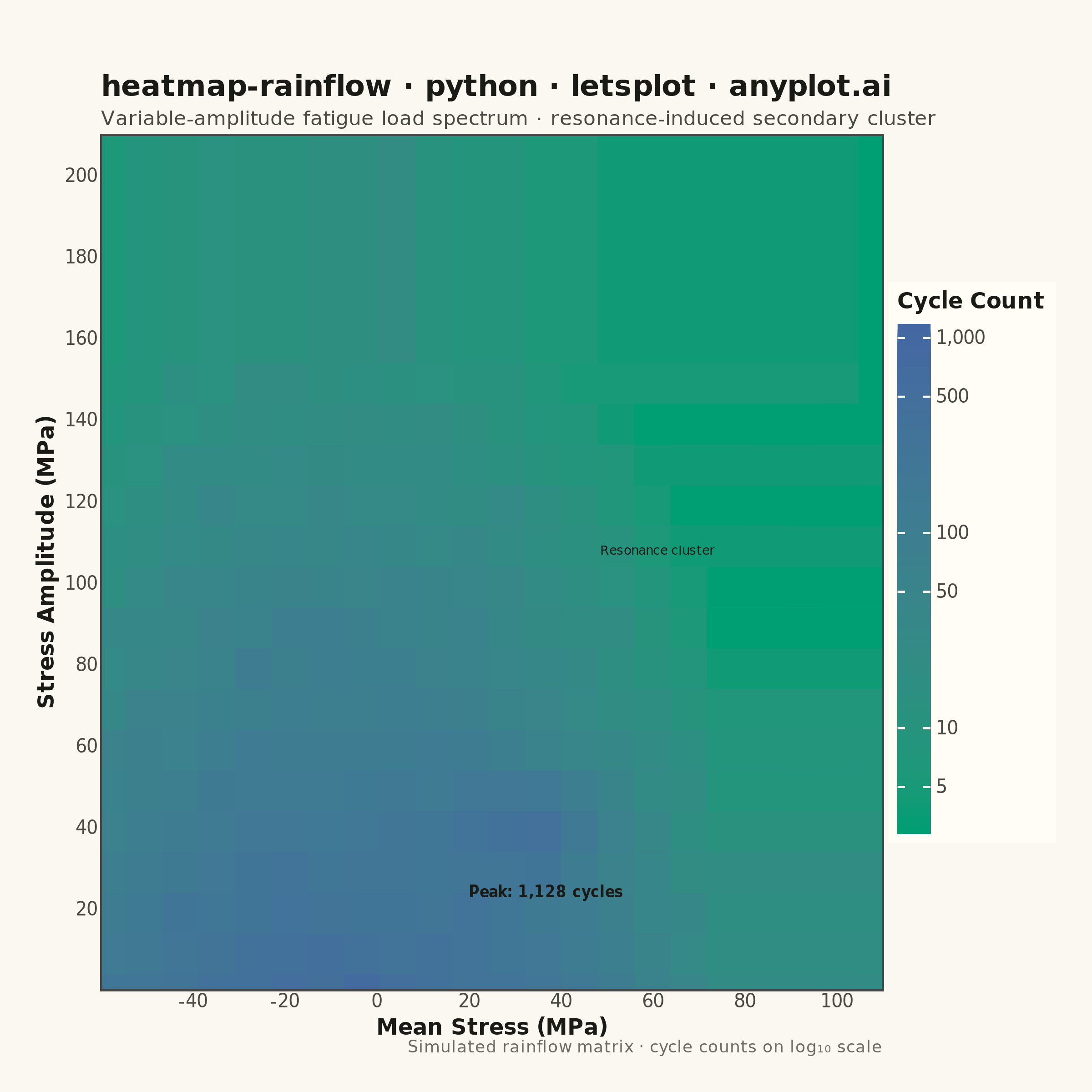
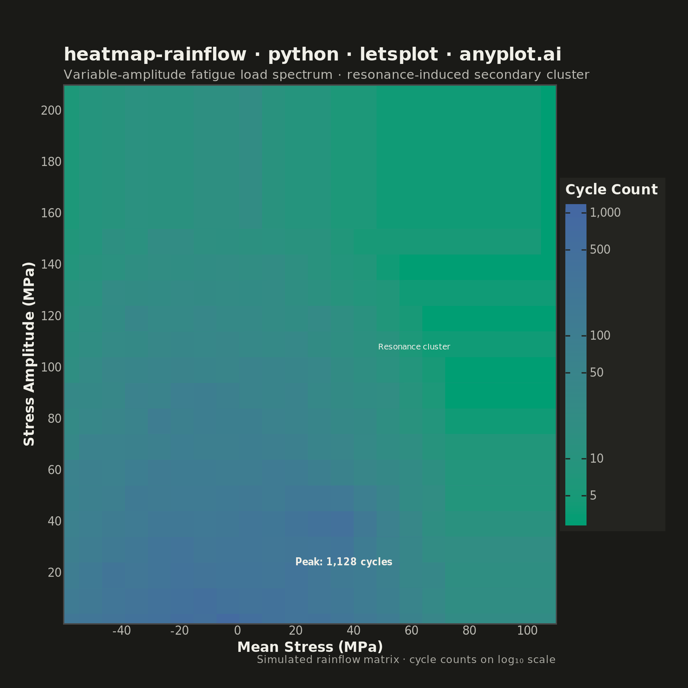
A rainflow counting matrix visualizes the results of rainflow cycle counting from a load or stress time history. The matrix displays cycle counts as a 2D heatmap where one axis represents cycle amplitude (half-range), the other represents cycle mean value, and color intensity represents the frequency of each cycle combination. This is a fundamental tool in fatigue analysis and durability engineering, used to characterize variable-amplitude loading for fatigue life prediction.
""" anyplot.ai
heatmap-rainflow: Rainflow Counting Matrix for Fatigue Analysis
Library: letsplot 4.10.1 | Python 3.13.13
Quality: 91/100 | Updated: 2026-06-02
"""

import os

import numpy as np
import pandas as pd
from lets_plot import (
    LetsPlot,
    aes,
    coord_cartesian,
    element_blank,
    element_line,
    element_rect,
    element_text,
    geom_text,
    geom_tile,
    ggplot,
    ggsize,
    guide_colorbar,
    labs,
    layer_tooltips,
    scale_fill_gradient,
    scale_x_continuous,
    scale_y_continuous,
    theme,
    theme_minimal,
)
from lets_plot.export import ggsave


LetsPlot.setup_html()

# Theme tokens — Imprint palette, theme-adaptive chrome
THEME = os.getenv("ANYPLOT_THEME", "light")
PAGE_BG = "#FAF8F1" if THEME == "light" else "#1A1A17"
ELEVATED_BG = "#FFFDF6" if THEME == "light" else "#242420"
INK = "#1A1A17" if THEME == "light" else "#F0EFE8"
INK_SOFT = "#4A4A44" if THEME == "light" else "#B8B7B0"
INK_MUTED = "#6B6A63" if THEME == "light" else "#A8A79F"

# Data — simulate rainflow counting from a variable-amplitude fatigue load signal
np.random.seed(42)

n_bins = 20
amplitude_centers = np.linspace(10, 200, n_bins)
mean_centers = np.linspace(-50, 100, n_bins)
amp_step = float(amplitude_centers[1] - amplitude_centers[0])
mean_step = float(mean_centers[1] - mean_centers[0])

# Realistic rainflow matrix: exponential decay in amplitude, Gaussian in mean
amp_grid, mean_grid = np.meshgrid(amplitude_centers, mean_centers, indexing="ij")
base_counts = 1000 * np.exp(-0.022 * amp_grid) * np.exp(-0.0004 * (mean_grid - 15) ** 2)
noise = np.random.exponential(scale=0.2, size=base_counts.shape)
raw_counts = np.round(base_counts * (1 + noise)).astype(int)

# Secondary cluster: resonance-induced loading at moderate amplitude / higher mean
resonance_amp = 80.0
resonance_mean = 55.0
secondary = 250 * np.exp(-0.008 * (amp_grid - resonance_amp) ** 2) * np.exp(-0.005 * (mean_grid - resonance_mean) ** 2)
raw_counts = raw_counts + np.round(secondary * (1 + noise * 0.3)).astype(int)
raw_counts[raw_counts < 3] = 0

# Build long-form DataFrame (only non-zero bins; zero bins show PAGE_BG background)
rows = []
for i, amp in enumerate(amplitude_centers):
    for j, mn in enumerate(mean_centers):
        count = raw_counts[i, j]
        if count > 0:
            rows.append({"amplitude": round(float(amp), 1), "mean_stress": round(float(mn), 1), "cycles": int(count)})

df = pd.DataFrame(rows)

# Pre-compute log10 for fill — gives stable gradient control with manual break labels
df["log_cycles"] = np.log10(df["cycles"].astype(float))
log_break_values = [5, 10, 50, 100, 500, 1000]
log_breaks = [np.log10(v) for v in log_break_values]
log_labels = ["5", "10", "50", "100", "500", "1,000"]

# Annotations — peak region and resonance cluster
peak_row = df.loc[df["cycles"].idxmax()]
peak_label = pd.DataFrame(
    {
        "mean_stress": [peak_row["mean_stress"]],
        "amplitude": [peak_row["amplitude"] + amp_step * 1.4],
        "label": [f"Peak: {int(peak_row['cycles']):,} cycles"],
    }
)
resonance_label = pd.DataFrame(
    {"mean_stress": [resonance_mean + 6], "amplitude": [resonance_amp + amp_step * 2.8], "label": ["Resonance cluster"]}
)

title = "heatmap-rainflow · python · letsplot · anyplot.ai"

# Plot — Imprint sequential colormap (green → blue) on log₁₀ scale
plot = (
    ggplot(df, aes(x="mean_stress", y="amplitude", fill="log_cycles"))
    + geom_tile(
        width=mean_step * 0.92,
        height=amp_step * 0.92,
        tooltips=layer_tooltips()
        .format("@amplitude", ".0f")
        .format("@mean_stress", ".0f")
        .format("@cycles", ",d")
        .line("Amplitude: @amplitude MPa")
        .line("Mean Stress: @mean_stress MPa")
        .line("Cycles: @cycles"),
    )
    + geom_text(
        aes(x="mean_stress", y="amplitude", label="label"),
        data=peak_label,
        inherit_aes=False,
        size=4,
        color=INK,
        fontface="bold",
    )
    + geom_text(
        aes(x="mean_stress", y="amplitude", label="label"), data=resonance_label, inherit_aes=False, size=3.5, color=INK
    )
    + scale_fill_gradient(
        low="#009E73",
        high="#4467A3",
        name="Cycle Count",
        breaks=log_breaks,
        labels=log_labels,
        guide=guide_colorbar(barwidth=18, barheight=280, nbin=256),
    )
    + scale_x_continuous(
        name="Mean Stress (MPa)", breaks=[-40, -20, 0, 20, 40, 60, 80, 100], format="d", expand=[0.02, 0]
    )
    + scale_y_continuous(
        name="Stress Amplitude (MPa)",
        breaks=[20, 40, 60, 80, 100, 120, 140, 160, 180, 200],
        format="d",
        expand=[0.02, 0],
    )
    + coord_cartesian(xlim=[-60, 110], ylim=[0, 210])
    + labs(
        title=title,
        subtitle="Variable-amplitude fatigue load spectrum · resonance-induced secondary cluster",
        caption="Simulated rainflow matrix · cycle counts on log₁₀ scale",
    )
    + theme_minimal()
    + theme(
        plot_background=element_rect(fill=PAGE_BG, color=PAGE_BG),
        panel_background=element_rect(fill=PAGE_BG),
        plot_title=element_text(size=16, face="bold", color=INK),
        plot_subtitle=element_text(size=11, color=INK_SOFT),
        plot_caption=element_text(size=9, color=INK_MUTED),
        axis_title=element_text(size=12, color=INK, face="bold"),
        axis_text=element_text(size=10, color=INK_SOFT),
        axis_line=element_line(color=INK_SOFT, size=0.5),
        legend_background=element_rect(fill=ELEVATED_BG, color=INK_SOFT),
        legend_text=element_text(size=10, color=INK_SOFT),
        legend_title=element_text(size=12, color=INK, face="bold"),
        panel_grid=element_blank(),
        plot_margin=[40, 20, 20, 20],
    )
    + ggsize(600, 600)
)

# Save
ggsave(plot, f"plot-{THEME}.png", path=".", scale=4)
ggsave(plot, f"plot-{THEME}.html", path=".")
Runnable source as JSON, for any HTTP client: https://api.anyplot.ai/specs/heatmap-rainflow/letsplot/code. Any spec id and library id listed in llms-full.txt fit the same URL shape; every URL below is complete and callable.
{
  "spec_id": "heatmap-rainflow",
  "language": "python",
  "library": "letsplot",
  "page": "https://anyplot.ai/heatmap-rainflow/python/letsplot",
  "hub": "https://anyplot.ai/heatmap-rainflow",
  "code_json": "https://api.anyplot.ai/specs/heatmap-rainflow/letsplot/code",
  "spec_json": "https://api.anyplot.ai/specs/heatmap-rainflow",
  "render_light_png": "https://storage.googleapis.com/anyplot-images/plots/heatmap-rainflow/python/letsplot/plot-light.png",
  "render_dark_png": "https://storage.googleapis.com/anyplot-images/plots/heatmap-rainflow/python/letsplot/plot-dark.png",
  "interactive_light_html": "https://storage.googleapis.com/anyplot-images/plots/heatmap-rainflow/python/letsplot/plot-light.html",
  "interactive_dark_html": "https://storage.googleapis.com/anyplot-images/plots/heatmap-rainflow/python/letsplot/plot-dark.html",
  "quality_score": 91.0,
  "license": "MIT",
  "guide": "https://anyplot.ai/llms.txt"
}
Part of Rainflow Counting Matrix for Fatigue Analysis on anyplot.ai.