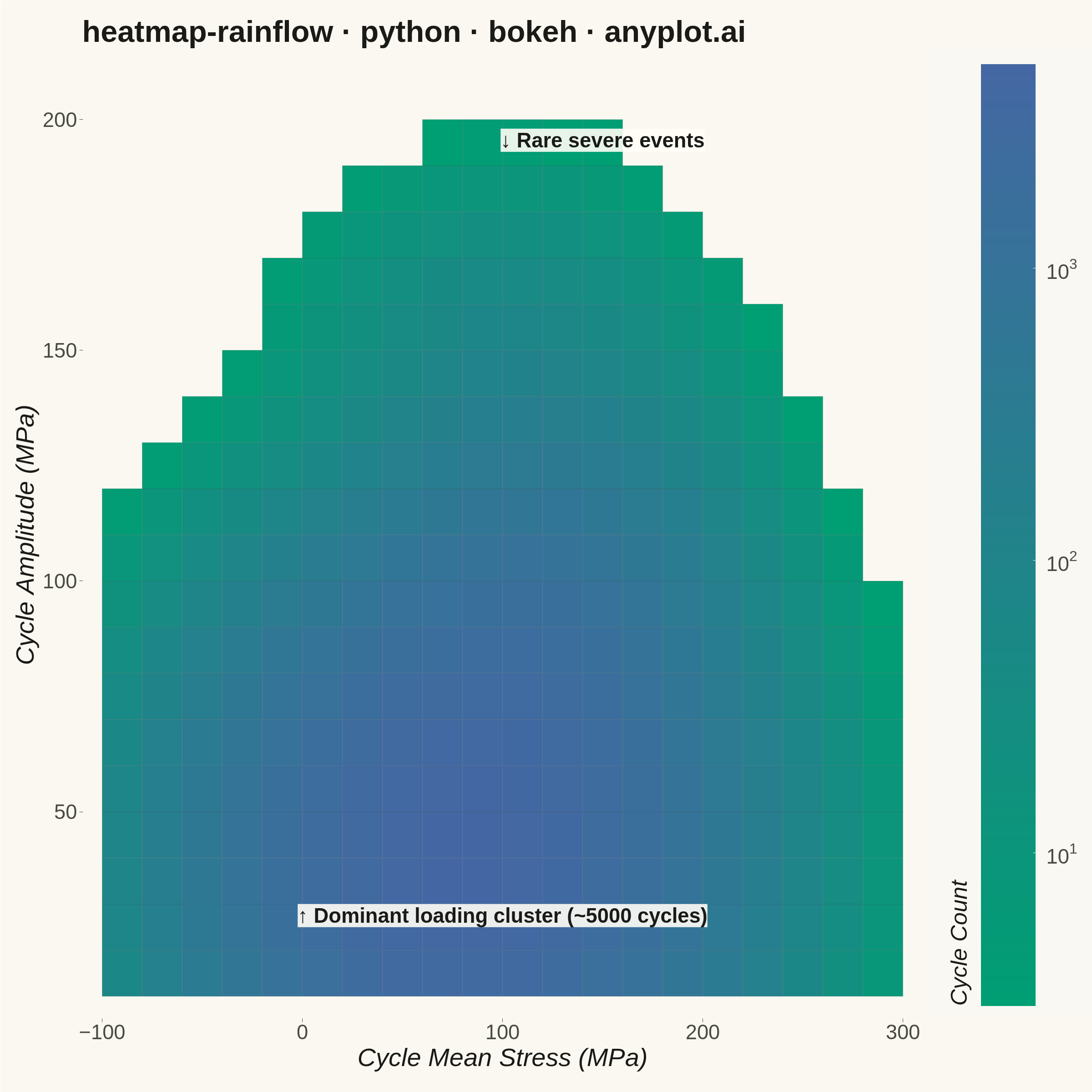
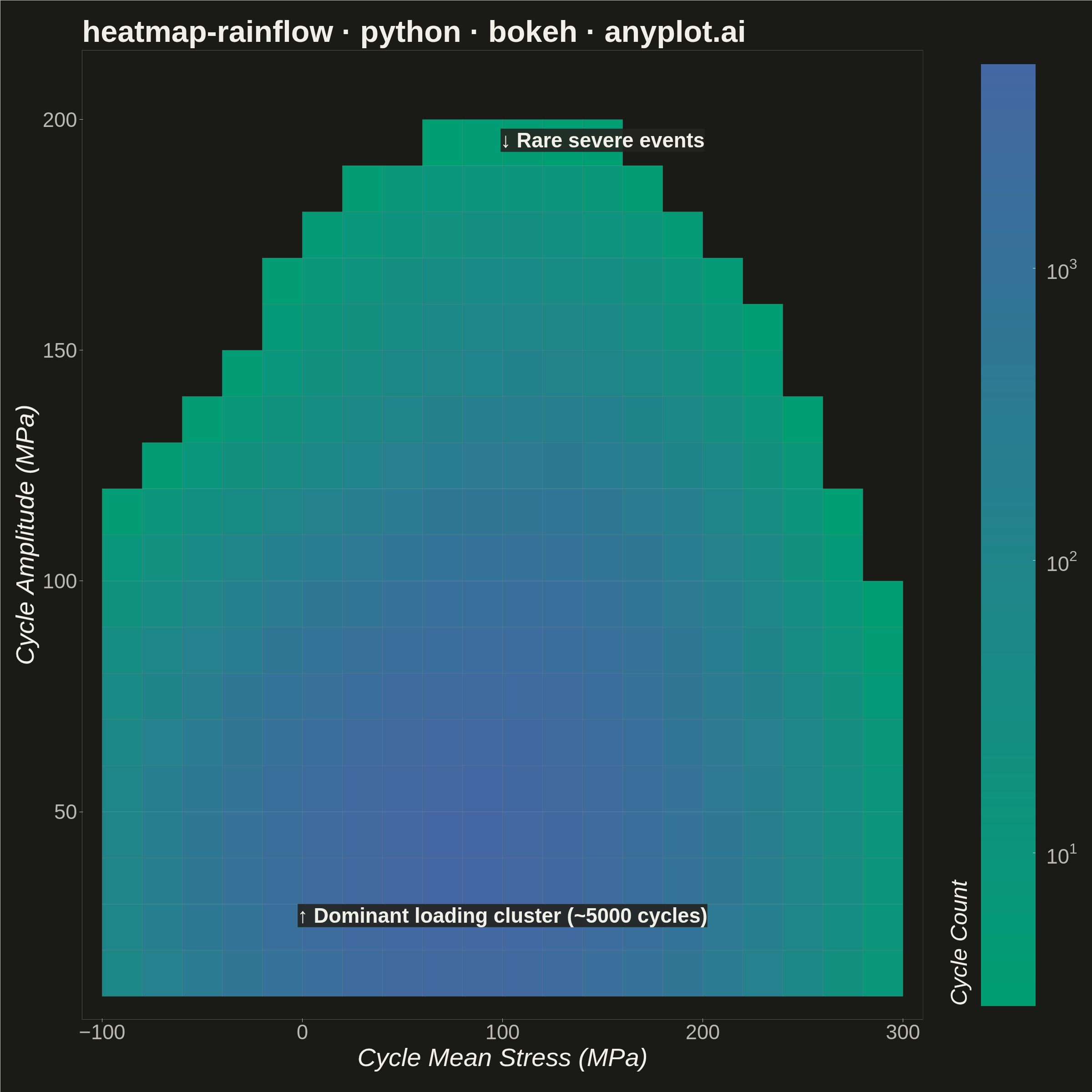
A rainflow counting matrix visualizes the results of rainflow cycle counting from a load or stress time history. The matrix displays cycle counts as a 2D heatmap where one axis represents cycle amplitude (half-range), the other represents cycle mean value, and color intensity represents the frequency of each cycle combination. This is a fundamental tool in fatigue analysis and durability engineering, used to characterize variable-amplitude loading for fatigue life prediction.
""" anyplot.ai
heatmap-rainflow: Rainflow Counting Matrix for Fatigue Analysis
Library: bokeh 3.9.0 | Python 3.13.13
Quality: 91/100 | Updated: 2026-06-02
"""

import os
import time
from pathlib import Path

import numpy as np
from bokeh.io import output_file, save
from bokeh.models import ColumnDataSource, HoverTool, Label, LogColorMapper, LogTicker
from bokeh.plotting import figure
from PIL import Image as _PILImage
from selenium import webdriver
from selenium.webdriver.chrome.options import Options


# Theme tokens — Imprint palette, theme-adaptive chrome
THEME = os.getenv("ANYPLOT_THEME", "light")
PAGE_BG = "#FAF8F1" if THEME == "light" else "#1A1A17"
ELEVATED_BG = "#FFFDF6" if THEME == "light" else "#242420"
INK = "#1A1A17" if THEME == "light" else "#F0EFE8"
INK_SOFT = "#4A4A44" if THEME == "light" else "#B8B7B0"

# Imprint sequential colormap: brand green → blue (256 stops, single-polarity counts)
_c0 = np.array([0x00, 0x9E, 0x73], dtype=float)  # #009E73
_c1 = np.array([0x44, 0x67, 0xA3], dtype=float)  # #4467A3
ANYPLOT_SEQ256 = ["#{:02X}{:02X}{:02X}".format(*np.round(_c0 + (_c1 - _c0) * t / 255).astype(int)) for t in range(256)]

# Data — Simulated rainflow counting matrix for a vehicle suspension component
np.random.seed(42)

n_bins = 20
amplitude_edges = np.linspace(10, 210, n_bins + 1)
mean_edges = np.linspace(-100, 300, n_bins + 1)
amplitude_centers = (amplitude_edges[:-1] + amplitude_edges[1:]) / 2
mean_centers = (mean_edges[:-1] + mean_edges[1:]) / 2

amplitude_grid, mean_grid = np.meshgrid(amplitude_centers, mean_centers, indexing="ij")

# Most cycles are low-amplitude near the mean load
cycle_density = np.exp(-0.5 * ((amplitude_grid - 40) / 30) ** 2 - 0.5 * ((mean_grid - 80) / 60) ** 2) * 5000
# Secondary cluster at moderate amplitude
cycle_density += np.exp(-0.5 * ((amplitude_grid - 90) / 25) ** 2 - 0.5 * ((mean_grid - 120) / 45) ** 2) * 800
# Sparse high-amplitude cycles (rare severe events)
cycle_density += np.exp(-0.5 * ((amplitude_grid - 150) / 20) ** 2 - 0.5 * ((mean_grid - 100) / 50) ** 2) * 50

cycle_counts = np.round(cycle_density).astype(int)
cycle_counts[cycle_counts < 3] = 0

# Numpy boolean indexing for non-zero bins
amp_idx, mean_idx = np.where(cycle_counts > 0)
amp_flat = amplitude_centers[amp_idx]
mean_flat = mean_centers[mean_idx]
count_flat = cycle_counts[amp_idx, mean_idx]

source = ColumnDataSource(
    data={
        "amplitude": amp_flat,
        "mean": mean_flat,
        "count": count_flat,
        "amp_label": [f"{v:.0f}" for v in amp_flat],
        "mean_label": [f"{v:.0f}" for v in mean_flat],
    }
)

amp_bin_width = float(amplitude_centers[1] - amplitude_centers[0])
mean_bin_width = float(mean_centers[1] - mean_centers[0])

# Log color mapper with Imprint sequential palette (wide count range needs log scale)
min_count = int(max(1, count_flat.min()))
max_count = int(count_flat.max())
color_mapper = LogColorMapper(palette=ANYPLOT_SEQ256, low=min_count, high=max_count, nan_color=PAGE_BG)

title = "heatmap-rainflow · python · bokeh · anyplot.ai"

# Plot — square 2400×2400 for symmetric heatmap
p = figure(
    width=2400,
    height=2400,
    title=title,
    x_axis_label="Cycle Mean Stress (MPa)",
    y_axis_label="Cycle Amplitude (MPa)",
    toolbar_location=None,
    tools="",
    x_range=(mean_edges[0] - mean_bin_width / 2, mean_edges[-1] + mean_bin_width / 2),
    y_range=(amplitude_edges[0] - amp_bin_width / 2, amplitude_edges[-1] + amp_bin_width / 2),
    min_border_bottom=160,
    min_border_left=180,
    min_border_top=110,
    min_border_right=200,
)

# Heatmap rectangles — thin cell border aids visual hierarchy at transition zones
r = p.rect(
    x="mean",
    y="amplitude",
    width=mean_bin_width,
    height=amp_bin_width,
    source=source,
    fill_color={"field": "count", "transform": color_mapper},
    line_color=INK_SOFT,
    line_alpha=0.2,
)

# Color bar — wider for 2400px canvas, theme-adaptive text
color_bar = r.construct_color_bar(
    width=120,
    ticker=LogTicker(),
    label_standoff=24,
    major_label_text_font_size="34pt",
    major_label_text_color=INK_SOFT,
    border_line_color=None,
    background_fill_color=PAGE_BG,
    padding=30,
    title="Cycle Count",
    title_text_font_size="38pt",
    title_text_color=INK,
    title_standoff=40,
)
p.add_layout(color_bar, "right")

# Hover tool for interactive HTML
hover = HoverTool(
    tooltips=[("Amplitude", "@amp_label MPa"), ("Mean", "@mean_label MPa"), ("Count", "@count")], renderers=[r]
)
p.add_tools(hover)

# Theme-adaptive chrome
p.background_fill_color = PAGE_BG
p.border_fill_color = PAGE_BG
p.outline_line_color = None

p.title.text_font_size = "50pt"
p.title.text_color = INK

p.xaxis.axis_label_text_font_size = "42pt"
p.yaxis.axis_label_text_font_size = "42pt"
p.xaxis.axis_label_text_color = INK
p.yaxis.axis_label_text_color = INK

p.xaxis.major_label_text_font_size = "34pt"
p.yaxis.major_label_text_font_size = "34pt"
p.xaxis.major_label_text_color = INK_SOFT
p.yaxis.major_label_text_color = INK_SOFT

p.xaxis.axis_line_color = None
p.yaxis.axis_line_color = None
p.xaxis.major_tick_line_color = INK_SOFT
p.yaxis.major_tick_line_color = INK_SOFT
p.axis.minor_tick_line_color = None

# No grid for clean heatmap aesthetic
p.xgrid.grid_line_color = None
p.ygrid.grid_line_color = None

# Annotations — storytelling guides viewer to dominant cluster and rare events (theme-adaptive)
dominant_label = Label(
    x=100,
    y=25,
    text="↑ Dominant loading cluster (~5000 cycles)",
    text_font_size="34pt",
    text_color=INK,
    text_font_style="bold",
    text_align="center",
    background_fill_color=ELEVATED_BG,
    background_fill_alpha=0.9,
)
p.add_layout(dominant_label)

# Rare events cluster is centered at amplitude ~150 MPa; label placed above it pointing down
rare_label = Label(
    x=150,
    y=193,
    text="↓ Rare severe events",
    text_font_size="34pt",
    text_color=INK,
    text_font_style="bold",
    text_align="center",
    background_fill_color=ELEVATED_BG,
    background_fill_alpha=0.9,
)
p.add_layout(rare_label)

# Save interactive HTML (catalog artifact)
output_file(f"plot-{THEME}.html")
save(p)

# Screenshot with headless Chrome — use CDP setDeviceMetricsOverride so the
# inner viewport is authoritative (--window-size alone is eaten by Chrome chrome
# in headless mode and gives ~139px less height than requested).
W, H = 2400, 2400
opts = Options()
for arg in (
    "--headless=new",
    "--no-sandbox",
    "--disable-dev-shm-usage",
    "--disable-gpu",
    f"--window-size={W},{H}",
    "--hide-scrollbars",
):
    opts.add_argument(arg)
driver = webdriver.Chrome(options=opts)
driver.execute_cdp_cmd(
    "Emulation.setDeviceMetricsOverride", {"width": W, "height": H, "deviceScaleFactor": 1, "mobile": False}
)
driver.get(f"file://{Path(f'plot-{THEME}.html').resolve()}")
time.sleep(3)
driver.save_screenshot(f"plot-{THEME}.png")
driver.quit()

# Belt-and-braces: pin the saved PNG to exact dims so the post-render gate passes
_img = _PILImage.open(f"plot-{THEME}.png").convert("RGB")
if _img.size != (W, H):
    _norm = _PILImage.new("RGB", (W, H), PAGE_BG)
    _norm.paste(_img, ((W - _img.size[0]) // 2, (H - _img.size[1]) // 2))
    _norm.save(f"plot-{THEME}.png")
Runnable source as JSON, for any HTTP client: https://api.anyplot.ai/specs/heatmap-rainflow/bokeh/code. Any spec id and library id listed in llms-full.txt fit the same URL shape; every URL below is complete and callable.
{
  "spec_id": "heatmap-rainflow",
  "language": "python",
  "library": "bokeh",
  "page": "https://anyplot.ai/heatmap-rainflow/python/bokeh",
  "hub": "https://anyplot.ai/heatmap-rainflow",
  "code_json": "https://api.anyplot.ai/specs/heatmap-rainflow/bokeh/code",
  "spec_json": "https://api.anyplot.ai/specs/heatmap-rainflow",
  "render_light_png": "https://storage.googleapis.com/anyplot-images/plots/heatmap-rainflow/python/bokeh/plot-light.png",
  "render_dark_png": "https://storage.googleapis.com/anyplot-images/plots/heatmap-rainflow/python/bokeh/plot-dark.png",
  "interactive_light_html": "https://storage.googleapis.com/anyplot-images/plots/heatmap-rainflow/python/bokeh/plot-light.html",
  "interactive_dark_html": "https://storage.googleapis.com/anyplot-images/plots/heatmap-rainflow/python/bokeh/plot-dark.html",
  "quality_score": 91.0,
  "license": "MIT",
  "guide": "https://anyplot.ai/llms.txt"
}
Part of Rainflow Counting Matrix for Fatigue Analysis on anyplot.ai.