The same plot in 14 other libraries — Python: Altair, Bokeh, lets-plot, Matplotlib, Plotly, plotnine, Pygal, Seaborn; R: ggplot2; JavaScript: Chart.js, D3.js, Apache ECharts, Highcharts, MUI X Charts. Compare all 15 side by side: Rainflow Counting Matrix for Fatigue Analysis in Python, R, Julia and JavaScript.
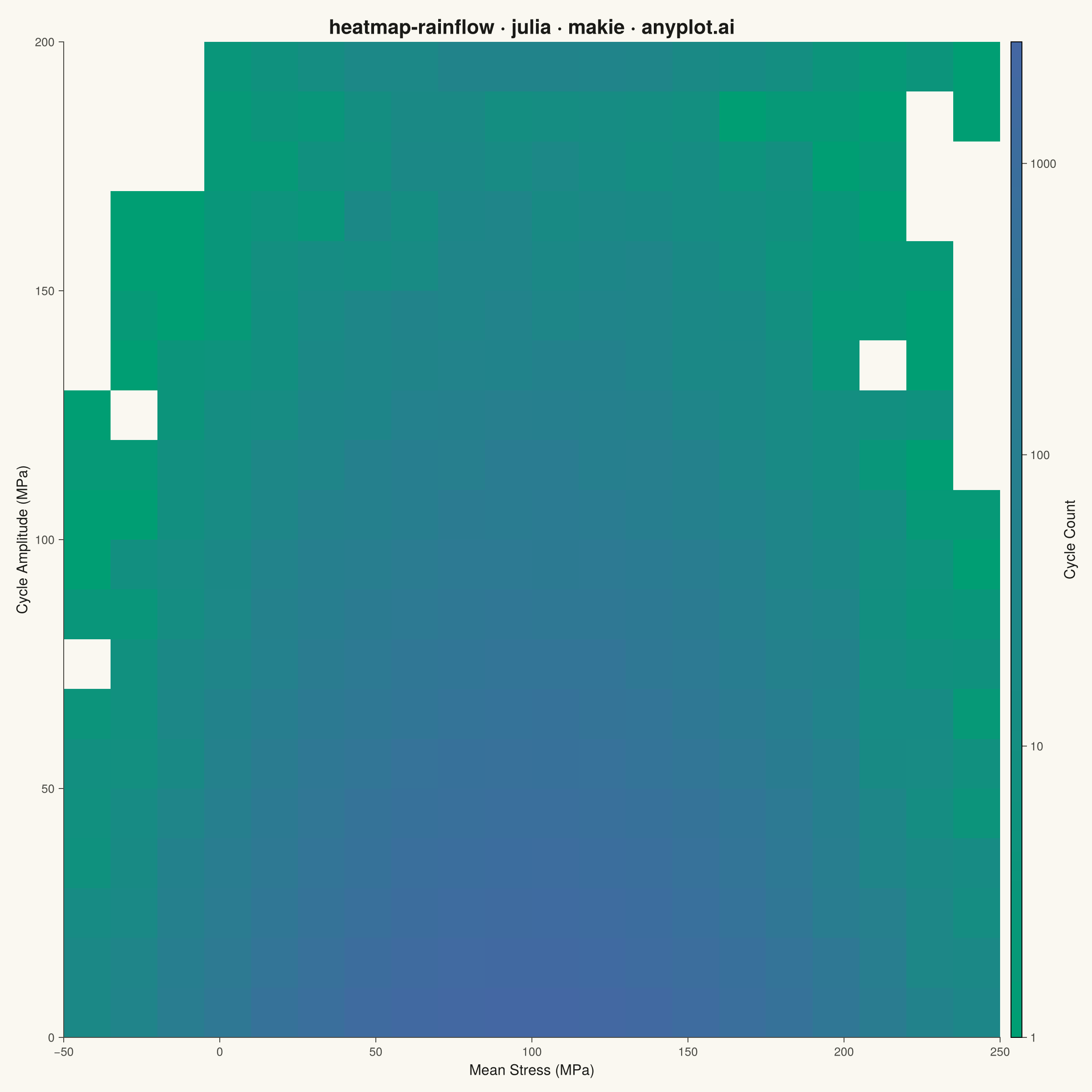
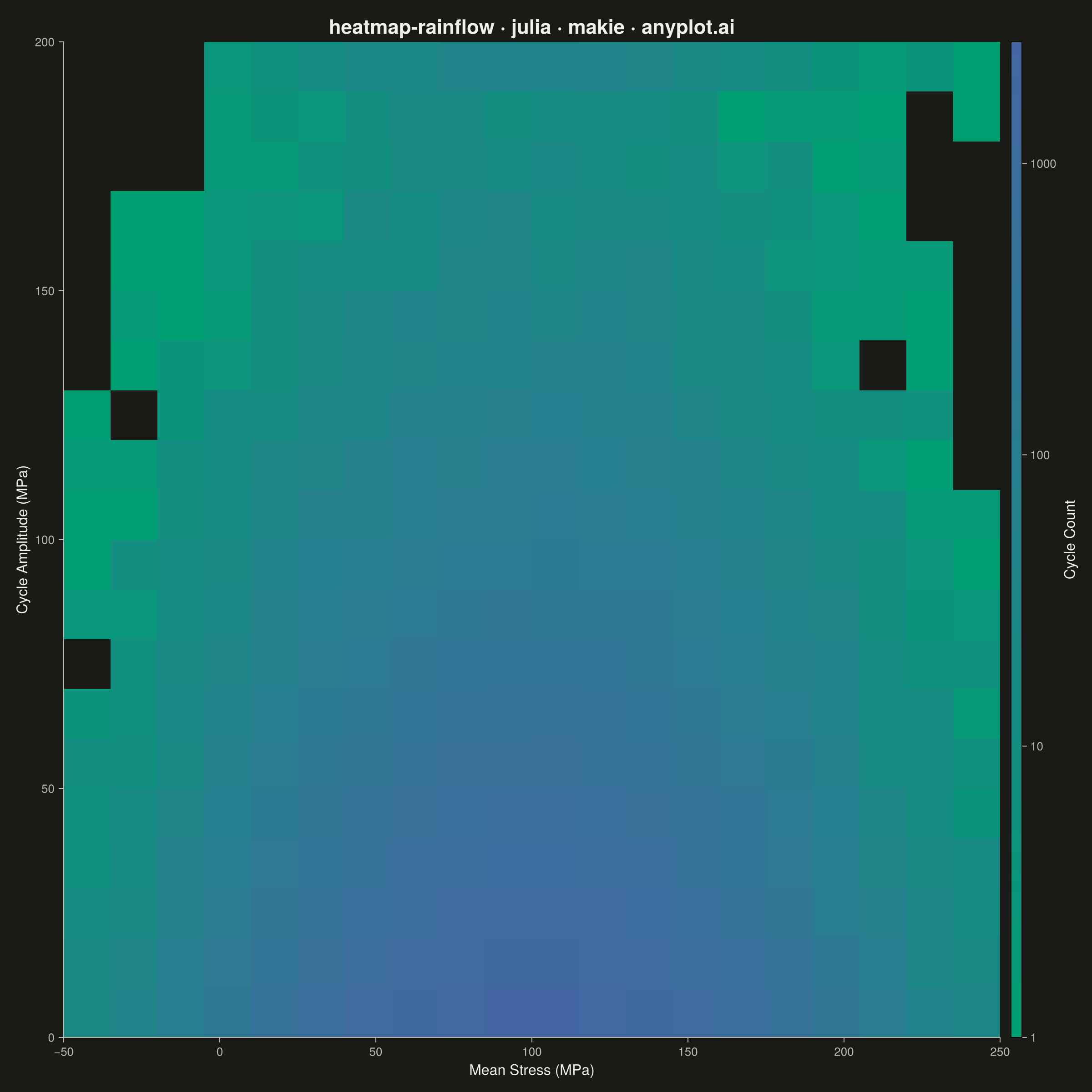
A rainflow counting matrix visualizes the results of rainflow cycle counting from a load or stress time history. The matrix displays cycle counts as a 2D heatmap where one axis represents cycle amplitude (half-range), the other represents cycle mean value, and color intensity represents the frequency of each cycle combination. This is a fundamental tool in fatigue analysis and durability engineering, used to characterize variable-amplitude loading for fatigue life prediction.
# anyplot.ai
# heatmap-rainflow: Rainflow Counting Matrix for Fatigue Analysis
# Library: makie 0.22.10 | Julia 1.11.9
# Quality: 85/100 | Created: 2026-06-02

using CairoMakie
using Colors
using Random

Random.seed!(42)

# Theme tokens
const THEME    = get(ENV, "ANYPLOT_THEME", "light")
const PAGE_BG  = THEME == "light" ? colorant"#FAF8F1" : colorant"#1A1A17"
const INK      = THEME == "light" ? colorant"#1A1A17" : colorant"#F0EFE8"
const INK_SOFT = THEME == "light" ? colorant"#4A4A44" : colorant"#B8B7B0"

# Imprint sequential colormap for single-polarity continuous data
const ANYPLOT_SEQ = cgrad([colorant"#009E73", colorant"#4467A3"])

# Data: variable-amplitude bridge loading — 200 000 cycles in a 20×20 rainflow matrix
n_amp  = 20
n_mean = 20

amp_min  = 0.0;   amp_max  = 200.0   # MPa
mean_min = -50.0; mean_max = 250.0   # MPa

amp_step  = (amp_max  - amp_min)  / n_amp
mean_step = (mean_max - mean_min) / n_mean

amp_centers  = [amp_min  + (i - 0.5) * amp_step  for i in 1:n_amp]
mean_centers = [mean_min + (i - 0.5) * mean_step for i in 1:n_mean]

n_cycles = 200_000
# Exponential amplitude distribution: physically realistic (many small, few large cycles)
amp_raw  = clamp.(-35.0 .* log.(rand(n_cycles)), amp_min + 1e-6, amp_max - 1e-6)
# Gaussian mean stress centred at 100 MPa (σ = 45 MPa)
mean_raw = clamp.(randn(n_cycles) .* 45.0 .+ 100.0, mean_min + 1e-6, mean_max - 1e-6)

amp_idx  = clamp.(ceil.(Int, (amp_raw  .- amp_min)  ./ amp_step),  1, n_amp)
mean_idx = clamp.(ceil.(Int, (mean_raw .- mean_min) ./ mean_step), 1, n_mean)

count_matrix = zeros(Int, n_amp, n_mean)
for k in 1:n_cycles
    count_matrix[amp_idx[k], mean_idx[k]] += 1
end

# Log10 transform; zero-count bins → NaN (rendered as background color)
count_display = Float64.(count_matrix)
count_display[count_matrix .== 0] .= NaN
count_log = log10.(count_display)

# Contour matrix: replace NaN with 0.0 so iso-lines trace the data boundary cleanly
count_log_contour = ifelse.(isnan.(count_log), 0.0, count_log)

valid_log = filter(!isnan, vec(count_log))
max_log   = isempty(valid_log) ? 1.0 : maximum(valid_log)

# Colorbar ticks at decade values within the data range
all_cb_counts = [1, 10, 100, 1_000, 10_000]
all_cb_vals   = log10.(Float64.(all_cb_counts))
keep          = all_cb_vals .<= max_log + 0.05
cb_vals       = all_cb_vals[keep]
cb_labels     = string.(all_cb_counts[keep])

# Centroid of the dominant fatigue zone (bins with ≥ 1 000 cycles)
high_mask = count_matrix .>= 1_000
cx_ann = 100.0  # default: Gaussian mean centre
cy_ann = 30.0   # default: low-amplitude region
if any(high_mask)
    total_w = Float64(sum(count_matrix[high_mask]))
    cx_ann  = sum(count_matrix[i, j] * mean_centers[j]
                  for i in 1:n_amp, j in 1:n_mean if high_mask[i, j]) / total_w
    cy_ann  = sum(count_matrix[i, j] * amp_centers[i]
                  for i in 1:n_amp, j in 1:n_mean if high_mask[i, j]) / total_w
end

# Figure: square canvas — 1200×1200 → 2400×2400 at px_per_unit=2
fig = Figure(
    size            = (1200, 1200),
    fontsize        = 14,
    backgroundcolor = PAGE_BG,
)

ax = Axis(
    fig[1, 1];
    title              = "Fatigue Spectrum · heatmap-rainflow · julia · makie · anyplot.ai",
    titlesize          = 19,
    titlecolor         = INK,
    xlabel             = "Mean Stress (MPa)",
    ylabel             = "Cycle Amplitude (MPa)",
    xlabelsize         = 16,
    ylabelsize         = 16,
    xticklabelsize     = 13,
    yticklabelsize     = 13,
    backgroundcolor    = PAGE_BG,
    topspinevisible    = false,
    rightspinevisible  = false,
    leftspinecolor     = INK_SOFT,
    bottomspinecolor   = INK_SOFT,
    xticklabelcolor    = INK_SOFT,
    yticklabelcolor    = INK_SOFT,
    xtickcolor         = INK_SOFT,
    ytickcolor         = INK_SOFT,
    xlabelcolor        = INK,
    ylabelcolor        = INK,
    xgridvisible       = false,
    ygridvisible       = false,
)

# heatmap!(ax, x, y, z): x → mean (cols), y → amplitude (rows); z must be (n_mean × n_amp)
hm = heatmap!(
    ax,
    mean_centers,
    amp_centers,
    count_log';
    colormap   = ANYPLOT_SEQ,
    nan_color  = PAGE_BG,
    colorrange = (0.0, max_log),
)

# Contour iso-lines at 100 and 1 000 cycles add visual hierarchy over the heatmap
contour!(
    ax,
    mean_centers,
    amp_centers,
    count_log_contour';
    levels    = [2.0, 3.0],
    color     = INK_SOFT,
    linewidth = 1.5,
)

# Annotate the dominant fatigue region centroid
text!(
    ax,
    cx_ann, cy_ann + 22.0;
    text     = "Dominant fatigue\nregion (>1k cycles/bin)",
    fontsize = 11,
    color    = INK,
    align    = (:center, :bottom),
)

cb = Colorbar(
    fig[1, 2],
    hm;
    label          = "Cycle Count",
    labelsize      = 16,
    labelcolor     = INK,
    ticklabelsize  = 13,
    ticklabelcolor = INK_SOFT,
    tickcolor      = INK_SOFT,
    ticks          = (cb_vals, cb_labels),
)

colgap!(fig.layout, 12)

save("plot-$(THEME).png", fig; px_per_unit = 2)
Runnable source as JSON, for any HTTP client: https://api.anyplot.ai/specs/heatmap-rainflow/makie/code. Any spec id and library id listed in llms-full.txt fit the same URL shape; every URL below is complete and callable.
{
  "spec_id": "heatmap-rainflow",
  "language": "julia",
  "library": "makie",
  "page": "https://anyplot.ai/heatmap-rainflow/julia/makie",
  "hub": "https://anyplot.ai/heatmap-rainflow",
  "code_json": "https://api.anyplot.ai/specs/heatmap-rainflow/makie/code",
  "spec_json": "https://api.anyplot.ai/specs/heatmap-rainflow",
  "render_light_png": "https://storage.googleapis.com/anyplot-images/plots/heatmap-rainflow/julia/makie/plot-light.png",
  "render_dark_png": "https://storage.googleapis.com/anyplot-images/plots/heatmap-rainflow/julia/makie/plot-dark.png",
  "quality_score": 85.0,
  "license": "MIT",
  "guide": "https://anyplot.ai/llms.txt"
}
Part of Rainflow Counting Matrix for Fatigue Analysis on anyplot.ai.