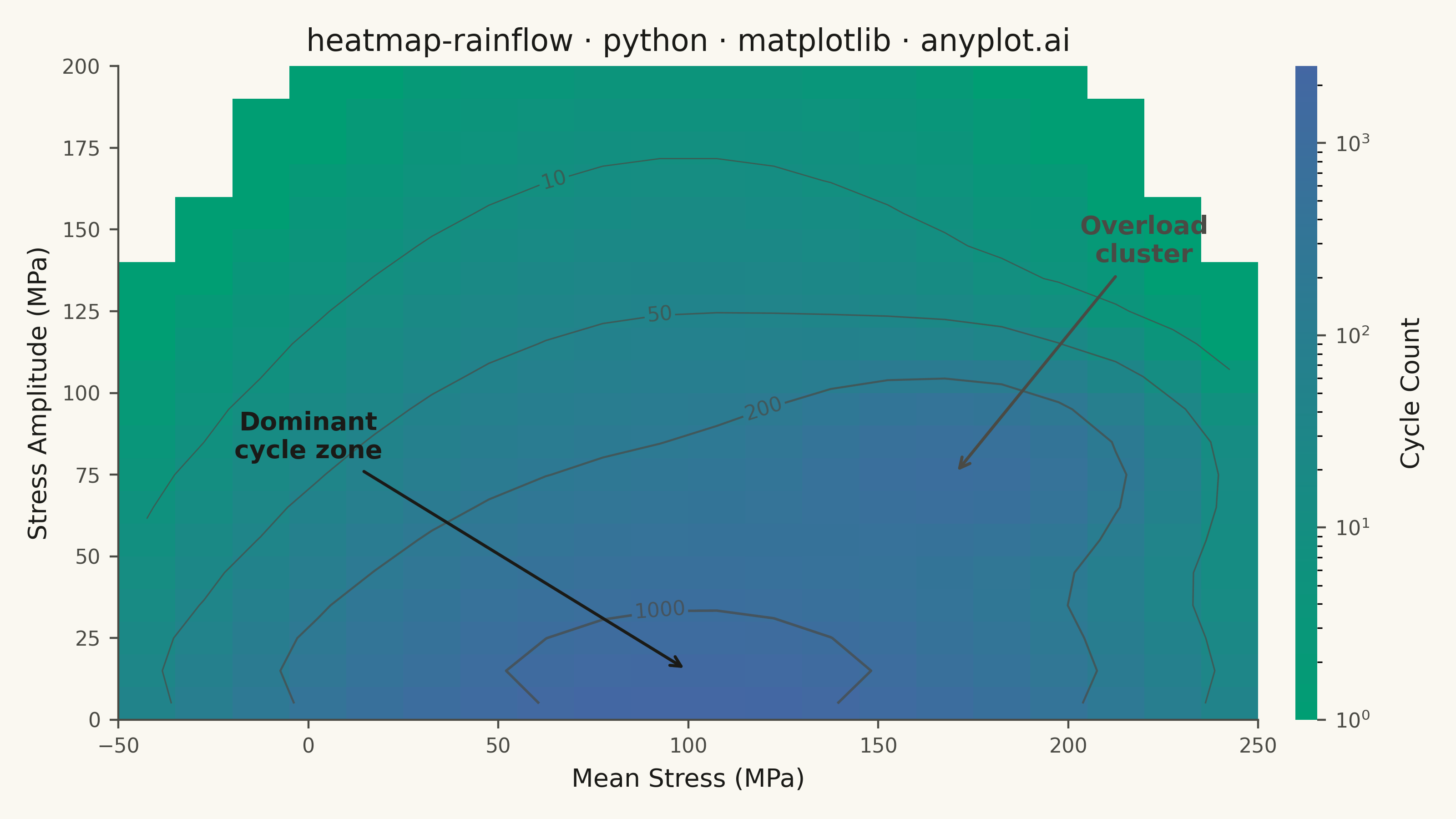
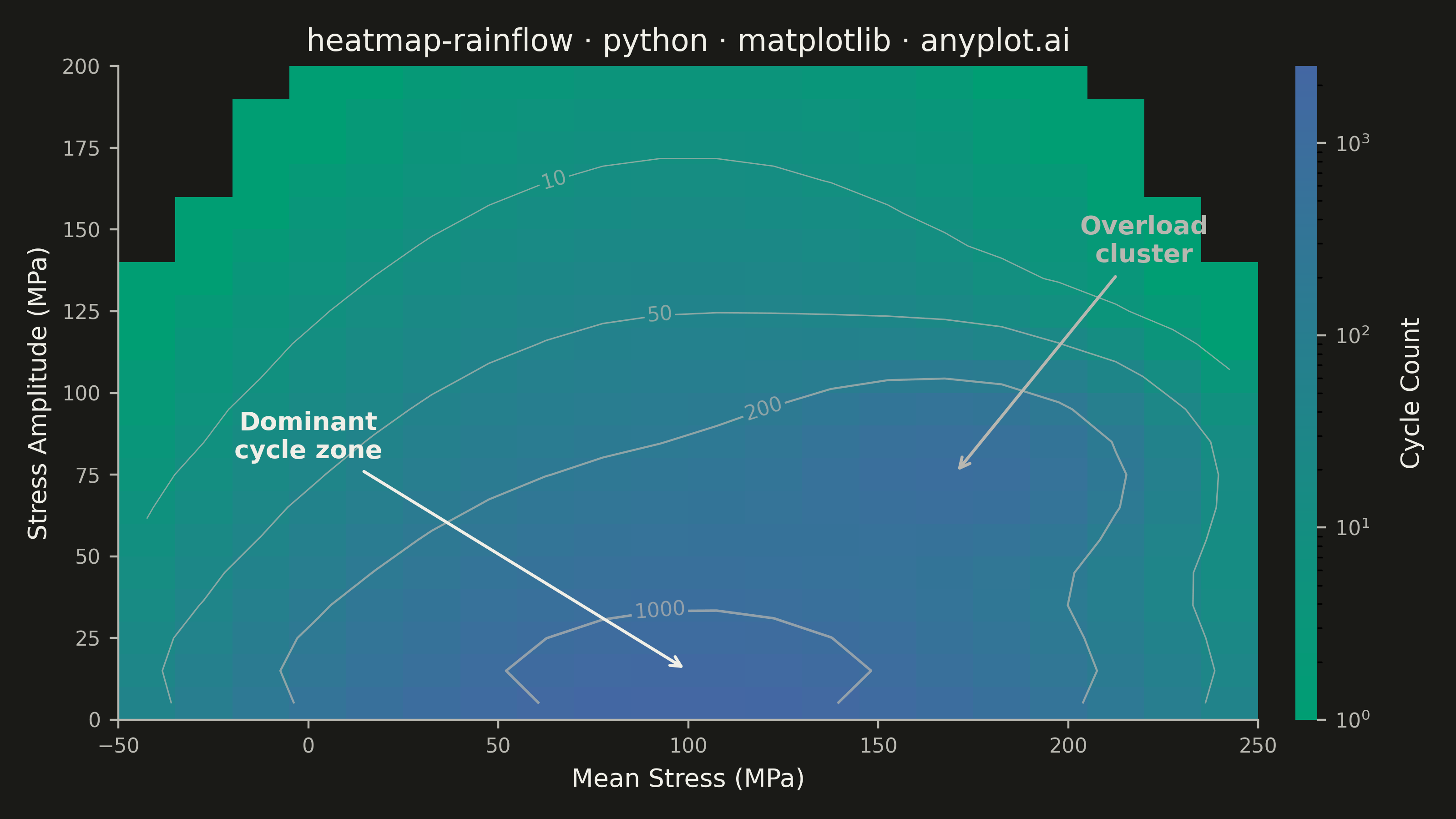
A rainflow counting matrix visualizes the results of rainflow cycle counting from a load or stress time history. The matrix displays cycle counts as a 2D heatmap where one axis represents cycle amplitude (half-range), the other represents cycle mean value, and color intensity represents the frequency of each cycle combination. This is a fundamental tool in fatigue analysis and durability engineering, used to characterize variable-amplitude loading for fatigue life prediction.
""" anyplot.ai
heatmap-rainflow: Rainflow Counting Matrix for Fatigue Analysis
Library: matplotlib 3.10.9 | Python 3.13.13
Quality: 93/100 | Updated: 2026-06-02
"""

import os

import matplotlib.pyplot as plt
import numpy as np
from matplotlib.colors import LinearSegmentedColormap, LogNorm
from matplotlib.ticker import LogFormatterSciNotation


# Theme tokens — Imprint palette, theme-adaptive chrome
THEME = os.getenv("ANYPLOT_THEME", "light")
PAGE_BG = "#FAF8F1" if THEME == "light" else "#1A1A17"
ELEVATED_BG = "#FFFDF6" if THEME == "light" else "#242420"
INK = "#1A1A17" if THEME == "light" else "#F0EFE8"
INK_SOFT = "#4A4A44" if THEME == "light" else "#B8B7B0"
INK_MUTED = "#6B6A63" if THEME == "light" else "#A8A79F"

# Imprint sequential colormap for continuous cycle-count data
imprint_seq = LinearSegmentedColormap.from_list("imprint_seq", ["#009E73", "#4467A3"])
imprint_seq.set_bad(PAGE_BG)  # masked zero-count bins blend with page background
imprint_seq.set_under(PAGE_BG)

# Data — simulate rainflow counting from variable-amplitude fatigue signal
np.random.seed(42)

n_amp_bins = 20
n_mean_bins = 20
amp_edges = np.linspace(0, 200, n_amp_bins + 1)
mean_edges = np.linspace(-50, 250, n_mean_bins + 1)
amp_centers = (amp_edges[:-1] + amp_edges[1:]) / 2
mean_centers = (mean_edges[:-1] + mean_edges[1:]) / 2

mean_grid, amp_grid = np.meshgrid(mean_centers, amp_centers)

# Dominant low-amplitude cycles near mean load (~100 MPa)
raw_counts = 3000 * np.exp(-amp_grid / 30) * np.exp(-((mean_grid - 100) ** 2) / (2 * 50**2))

# Secondary overload cluster at higher amplitude
raw_counts += 800 * np.exp(-((amp_grid - 75) ** 2) / (2 * 15**2)) * np.exp(-((mean_grid - 170) ** 2) / (2 * 25**2))

cycle_counts = np.clip(np.round(raw_counts).astype(int), 0, None)
masked_counts = np.ma.masked_where(cycle_counts == 0, cycle_counts)

# Gaussian-smoothed counts for contour overlay
k = np.arange(-3, 4)
kernel_1d = np.exp(-0.5 * (k / 1.2) ** 2)
kernel_1d /= kernel_1d.sum()
smooth_counts = np.apply_along_axis(lambda r: np.convolve(r, kernel_1d, mode="same"), 0, cycle_counts.astype(float))
smooth_counts = np.apply_along_axis(lambda r: np.convolve(r, kernel_1d, mode="same"), 1, smooth_counts)

# Plot
title = "heatmap-rainflow · python · matplotlib · anyplot.ai"
title_fontsize = max(8, round(12 * 67 / len(title))) if len(title) > 67 else 12

fig, ax = plt.subplots(figsize=(8, 4.5), dpi=400, facecolor=PAGE_BG)
ax.set_facecolor(PAGE_BG)

im = ax.pcolormesh(
    mean_edges,
    amp_edges,
    masked_counts,
    cmap=imprint_seq,
    norm=LogNorm(vmin=1, vmax=cycle_counts.max()),
    shading="flat",
)

# Contour threshold overlay — quantitative reference lines
contour_levels = [10, 50, 200, 1000]
cs = ax.contour(
    mean_centers,
    amp_centers,
    smooth_counts,
    levels=contour_levels,
    colors=INK_SOFT,
    linewidths=[0.5, 0.6, 0.8, 1.0],
    alpha=0.7,
)
ax.clabel(cs, inline=True, fontsize=8, fmt="%d", colors=INK_SOFT)

# Colorbar
cbar = fig.colorbar(im, ax=ax, fraction=0.046, pad=0.03, aspect=30)
cbar.ax.tick_params(labelsize=8, colors=INK_SOFT)
cbar.ax.yaxis.set_major_formatter(LogFormatterSciNotation(minor_thresholds=(2, 0.5)))
cbar.set_label("Cycle Count", fontsize=10, labelpad=12, color=INK)
cbar.outline.set_visible(False)

# Annotations — highlight dominant zone and overload cluster
ax.annotate(
    "Dominant\ncycle zone",
    xy=(100, 15),
    xytext=(0, 80),
    fontsize=10,
    fontweight="bold",
    color=INK,
    ha="center",
    arrowprops={"arrowstyle": "->", "color": INK, "lw": 1.2},
)
ax.annotate(
    "Overload\ncluster",
    xy=(170, 75),
    xytext=(220, 140),
    fontsize=10,
    fontweight="bold",
    color=INK_SOFT,
    ha="center",
    arrowprops={"arrowstyle": "->", "color": INK_SOFT, "lw": 1.2},
)

# Style — theme-adaptive chrome
ax.set_xlabel("Mean Stress (MPa)", fontsize=10, color=INK)
ax.set_ylabel("Stress Amplitude (MPa)", fontsize=10, color=INK)
ax.set_title(title, fontsize=title_fontsize, fontweight="medium", color=INK)
ax.tick_params(axis="both", labelsize=8, colors=INK_SOFT)
ax.spines["top"].set_visible(False)
ax.spines["right"].set_visible(False)
for s in ("left", "bottom"):
    ax.spines[s].set_color(INK_SOFT)

fig.tight_layout()
plt.savefig(f"plot-{THEME}.png", dpi=400, facecolor=PAGE_BG)
Runnable source as JSON, for any HTTP client: https://api.anyplot.ai/specs/heatmap-rainflow/matplotlib/code. Any spec id and library id listed in llms-full.txt fit the same URL shape; every URL below is complete and callable.
{
  "spec_id": "heatmap-rainflow",
  "language": "python",
  "library": "matplotlib",
  "page": "https://anyplot.ai/heatmap-rainflow/python/matplotlib",
  "hub": "https://anyplot.ai/heatmap-rainflow",
  "code_json": "https://api.anyplot.ai/specs/heatmap-rainflow/matplotlib/code",
  "spec_json": "https://api.anyplot.ai/specs/heatmap-rainflow",
  "render_light_png": "https://storage.googleapis.com/anyplot-images/plots/heatmap-rainflow/python/matplotlib/plot-light.png",
  "render_dark_png": "https://storage.googleapis.com/anyplot-images/plots/heatmap-rainflow/python/matplotlib/plot-dark.png",
  "quality_score": 93.0,
  "license": "MIT",
  "guide": "https://anyplot.ai/llms.txt"
}
Part of Rainflow Counting Matrix for Fatigue Analysis on anyplot.ai.