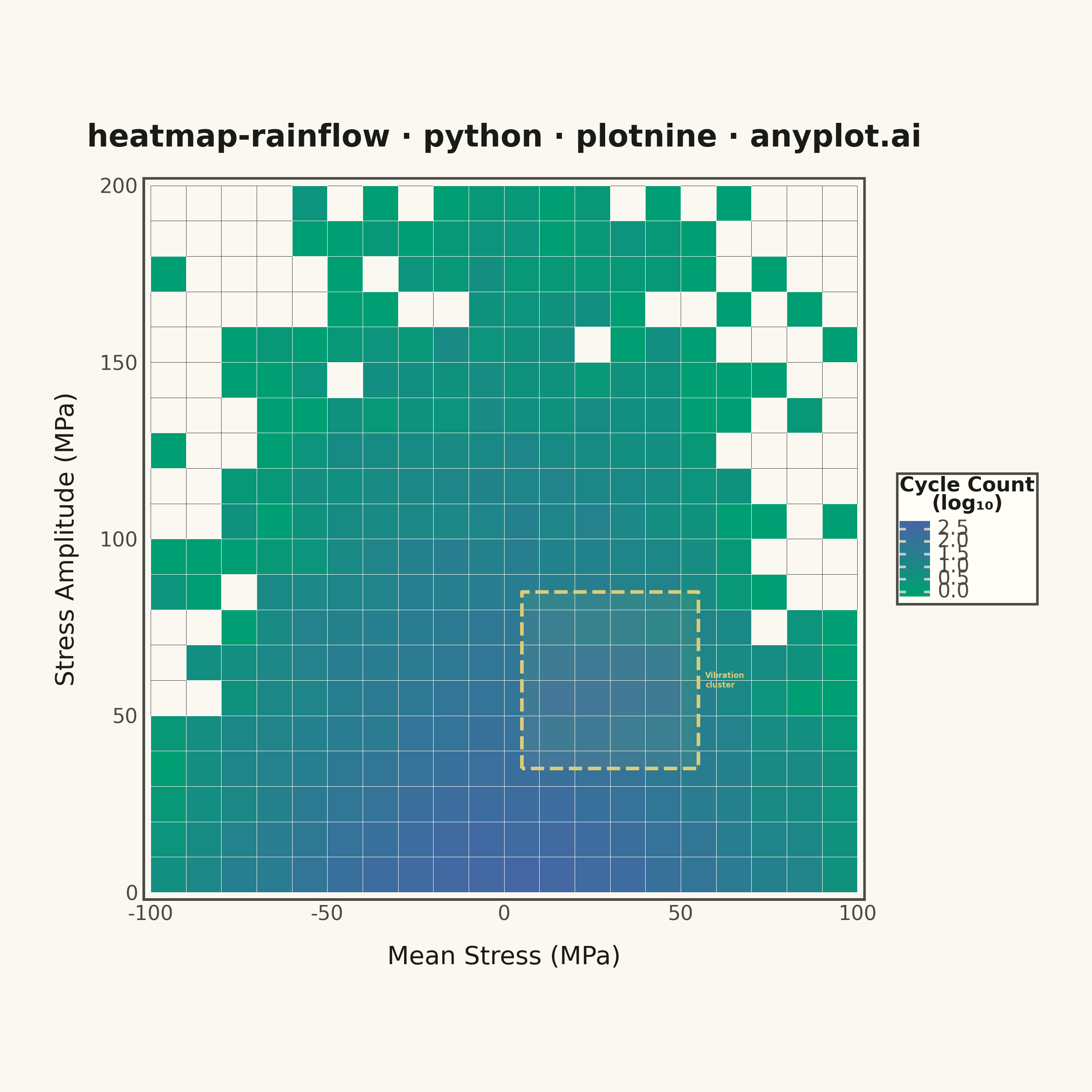
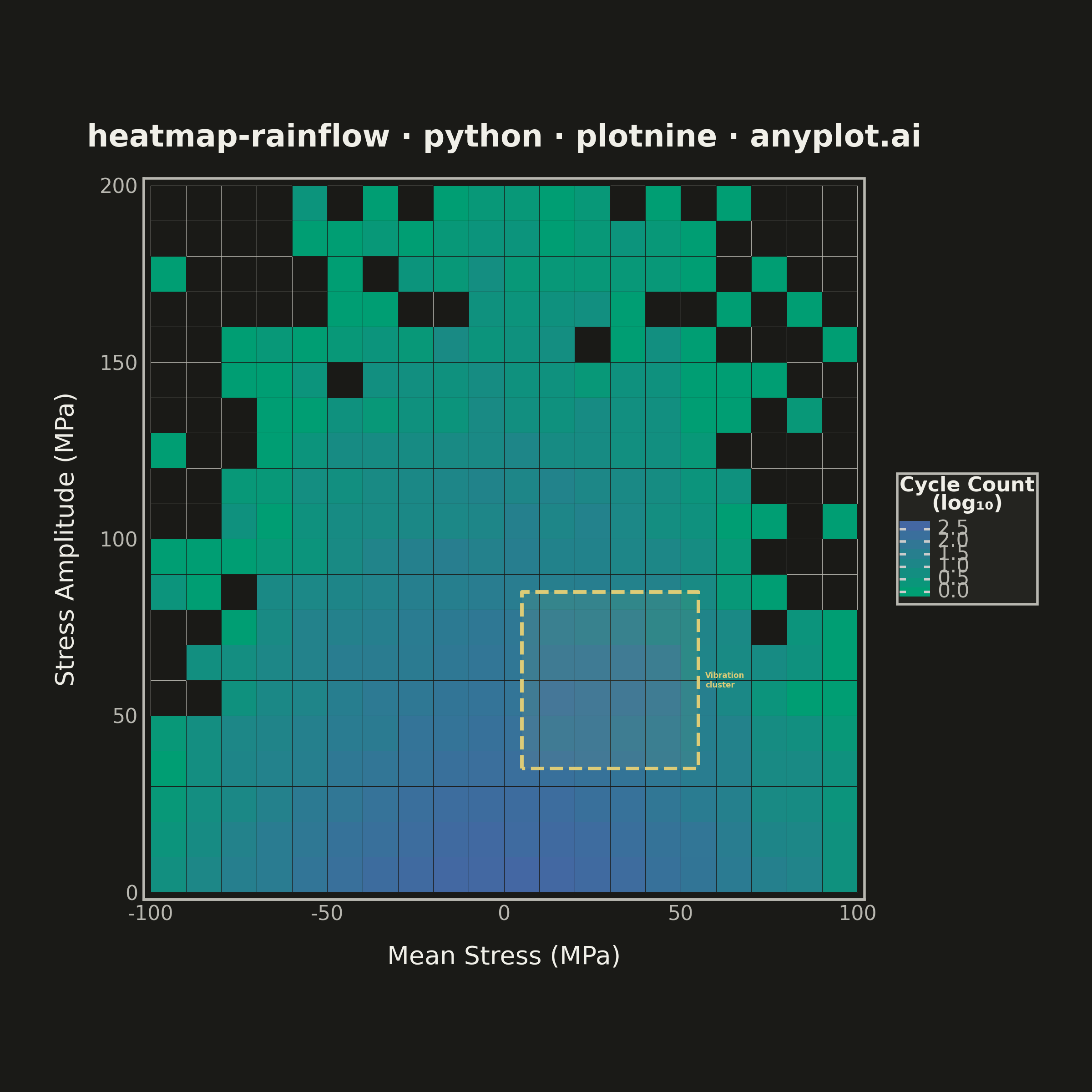
A rainflow counting matrix visualizes the results of rainflow cycle counting from a load or stress time history. The matrix displays cycle counts as a 2D heatmap where one axis represents cycle amplitude (half-range), the other represents cycle mean value, and color intensity represents the frequency of each cycle combination. This is a fundamental tool in fatigue analysis and durability engineering, used to characterize variable-amplitude loading for fatigue life prediction.
""" anyplot.ai
heatmap-rainflow: Rainflow Counting Matrix for Fatigue Analysis
Library: plotnine 0.15.4 | Python 3.13.13
Quality: 90/100 | Updated: 2026-06-02
"""

import os
import sys

import numpy as np
import pandas as pd


# Work around naming conflict with plotnine.py script and plotnine package
script_dir = os.path.dirname(os.path.abspath(__file__))
if script_dir in sys.path:
    sys.path.remove(script_dir)
if "" in sys.path:
    sys.path.remove("")
if "." in sys.path:
    sys.path.remove(".")

from plotnine import (
    aes,
    annotate,
    coord_fixed,
    element_blank,
    element_line,
    element_rect,
    element_text,
    geom_tile,
    ggplot,
    guide_colorbar,
    guides,
    labs,
    scale_fill_gradient,
    scale_x_continuous,
    scale_y_continuous,
    theme,
    theme_minimal,
)


# Theme tokens — Imprint palette chrome
THEME = os.getenv("ANYPLOT_THEME", "light")
PAGE_BG = "#FAF8F1" if THEME == "light" else "#1A1A17"
ELEVATED_BG = "#FFFDF6" if THEME == "light" else "#242420"
INK = "#1A1A17" if THEME == "light" else "#F0EFE8"
INK_SOFT = "#4A4A44" if THEME == "light" else "#B8B7B0"
ANYPLOT_AMBER = "#DDCC77"  # caution anchor — secondary cluster annotation

# Data — simulate rainflow counting results from variable-amplitude loading
np.random.seed(42)

n_amp_bins = 20
n_mean_bins = 20
amplitude_edges = np.linspace(0, 200, n_amp_bins + 1)
mean_edges = np.linspace(-100, 100, n_mean_bins + 1)
amplitude_centers = (amplitude_edges[:-1] + amplitude_edges[1:]) / 2
mean_centers = (mean_edges[:-1] + mean_edges[1:]) / 2

# Build rainflow matrix: most cycles at low amplitude near zero mean
amp_grid, mean_grid = np.meshgrid(amplitude_centers, mean_centers, indexing="ij")
cycle_rate = np.exp(-0.03 * amp_grid) * np.exp(-0.0005 * mean_grid**2)
cycle_counts = np.random.poisson(lam=cycle_rate * 500)

# Secondary cluster at moderate amplitude / positive mean (realistic loading)
cluster = 80 * np.exp(-0.01 * (amp_grid - 60) ** 2 - 0.002 * (mean_grid - 30) ** 2)
cycle_counts += np.random.poisson(lam=cluster)

# Build long-form DataFrame via vectorized numpy array flattening
df = pd.DataFrame(
    {
        "Amplitude (MPa)": amp_grid.flatten(),
        "Mean Stress (MPa)": mean_grid.flatten(),
        "Cycle Count": cycle_counts.flatten(),
    }
)

tile_w = float(mean_centers[1] - mean_centers[0])
tile_h = float(amplitude_centers[1] - amplitude_centers[0])

# Separate zero and nonzero for visual distinction
df_nonzero = df[df["Cycle Count"] > 0].copy()
df_nonzero["Log Count"] = np.log10(df_nonzero["Cycle Count"])

# Plot
plot = (
    ggplot()
    # Layer 1: Background-colored tiles for zero-count bins (visually distinct)
    + geom_tile(
        data=df,
        mapping=aes(x="Mean Stress (MPa)", y="Amplitude (MPa)"),
        fill=PAGE_BG,
        color=INK_SOFT,
        size=0.1,
        width=tile_w,
        height=tile_h,
        alpha=0.4,
    )
    # Layer 2: Imprint sequential gradient for nonzero bins
    + geom_tile(
        data=df_nonzero,
        mapping=aes(x="Mean Stress (MPa)", y="Amplitude (MPa)", fill="Log Count"),
        color=PAGE_BG,
        size=0.1,
        width=tile_w,
        height=tile_h,
    )
    # Imprint sequential colormap: brand green → blue (single-polarity count data)
    + scale_fill_gradient(
        low="#009E73", high="#4467A3", name="Cycle Count\n(log₁₀)", limits=(0, df_nonzero["Log Count"].max())
    )
    # Advanced plotnine: stepped colorbar with discrete rectangles (nbin steps)
    + guides(fill=guide_colorbar(nbin=8, display="rectangles", draw_ulim=True, draw_llim=True))
    # Highlight the secondary vibration-loading cluster (~60 MPa amp / +30 MPa mean)
    + annotate(
        "rect",
        xmin=5.0,
        xmax=55.0,
        ymin=35.0,
        ymax=85.0,
        fill=ANYPLOT_AMBER,
        color=ANYPLOT_AMBER,
        size=0.8,
        linetype="dashed",
        alpha=0.08,
    )
    + annotate(
        "text", x=57.0, y=60.0, label="Vibration\ncluster", color=ANYPLOT_AMBER, size=3.0, ha="left", fontweight="bold"
    )
    # coord_fixed: enforces square cells for symmetric amplitude/mean-stress ranges
    + coord_fixed(ratio=1)
    + scale_x_continuous(expand=(0, 2))
    + scale_y_continuous(expand=(0, 2))
    + labs(x="Mean Stress (MPa)", y="Stress Amplitude (MPa)", title="heatmap-rainflow · python · plotnine · anyplot.ai")
    + theme_minimal()
    + theme(
        figure_size=(6, 6),
        text=element_text(family="sans-serif"),
        plot_title=element_text(size=12, ha="center", weight="bold", color=INK, margin={"b": 10}),
        axis_title_x=element_text(size=10, color=INK, margin={"t": 8}),
        axis_title_y=element_text(size=10, color=INK, margin={"r": 8}),
        axis_text_x=element_text(size=8, color=INK_SOFT),
        axis_text_y=element_text(size=8, color=INK_SOFT),
        axis_line=element_line(color=INK_SOFT),
        legend_title=element_text(size=8, weight="bold", color=INK),
        legend_text=element_text(size=8, color=INK_SOFT),
        legend_position="right",
        legend_key_height=30,
        legend_key_width=12,
        legend_background=element_rect(fill=ELEVATED_BG, color=INK_SOFT),
        panel_grid_major=element_blank(),
        panel_grid_minor=element_blank(),
        panel_border=element_rect(color=INK_SOFT, fill=None),
        panel_background=element_rect(fill=PAGE_BG),
        plot_background=element_rect(fill=PAGE_BG, color=PAGE_BG),
        plot_margin=0.05,
    )
)

plot.save(f"plot-{THEME}.png", dpi=400, width=6, height=6, units="in", verbose=False)
Runnable source as JSON, for any HTTP client: https://api.anyplot.ai/specs/heatmap-rainflow/plotnine/code. Any spec id and library id listed in llms-full.txt fit the same URL shape; every URL below is complete and callable.
{
  "spec_id": "heatmap-rainflow",
  "language": "python",
  "library": "plotnine",
  "page": "https://anyplot.ai/heatmap-rainflow/python/plotnine",
  "hub": "https://anyplot.ai/heatmap-rainflow",
  "code_json": "https://api.anyplot.ai/specs/heatmap-rainflow/plotnine/code",
  "spec_json": "https://api.anyplot.ai/specs/heatmap-rainflow",
  "render_light_png": "https://storage.googleapis.com/anyplot-images/plots/heatmap-rainflow/python/plotnine/plot-light.png",
  "render_dark_png": "https://storage.googleapis.com/anyplot-images/plots/heatmap-rainflow/python/plotnine/plot-dark.png",
  "quality_score": 90.0,
  "license": "MIT",
  "guide": "https://anyplot.ai/llms.txt"
}
Part of Rainflow Counting Matrix for Fatigue Analysis on anyplot.ai.