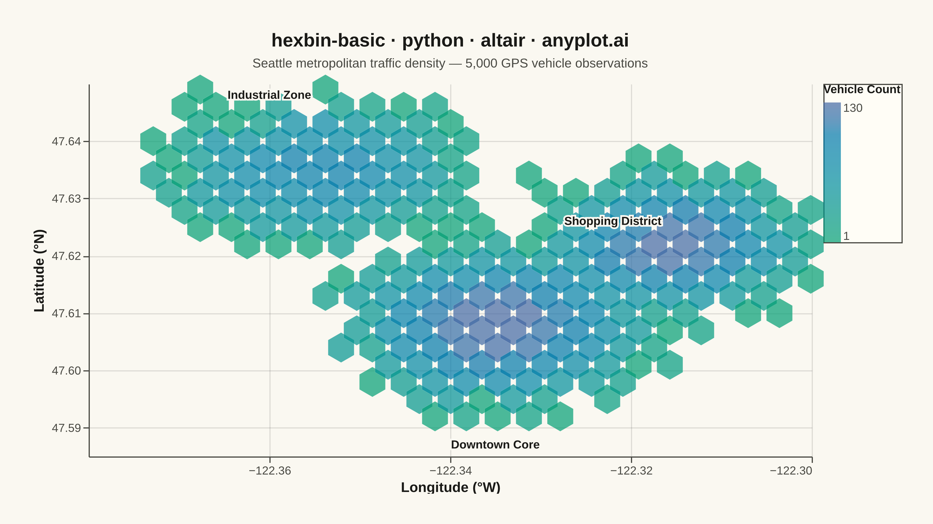
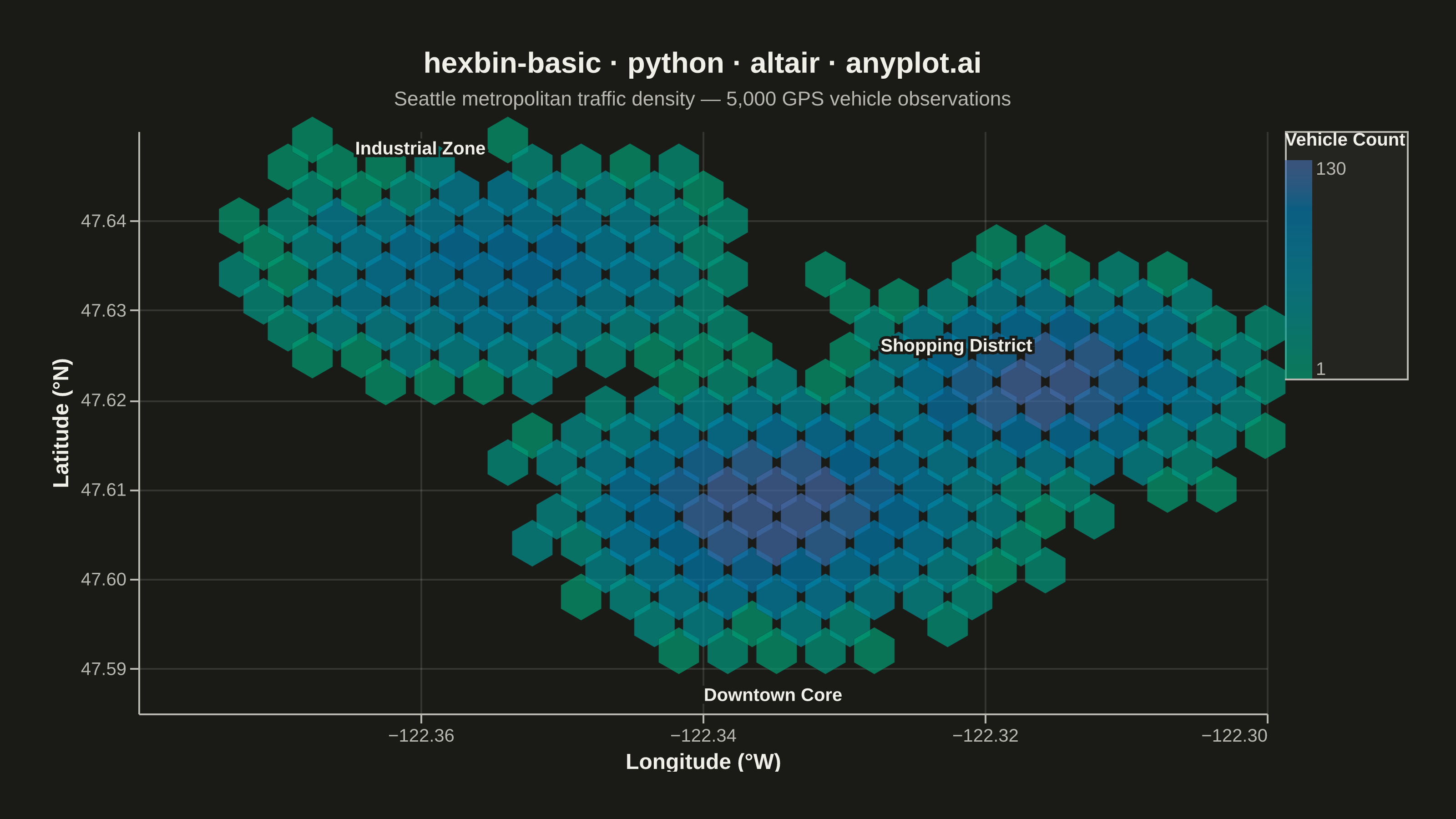
A hexagonal binning plot that visualizes the density of 2D point data by aggregating points into hexagonal bins. The color intensity of each hexagon represents the count of points within it, making it ideal for revealing density patterns in large datasets where traditional scatter plots would show overlapping points. Hexagonal bins provide better visual representation than square pixels due to their isotropy (equal distance to neighboring cells in all directions).
""" anyplot.ai
hexbin-basic: Basic Hexbin Plot
Library: altair 6.1.0 | Python 3.13.13
Quality: 88/100 | Updated: 2026-05-29
"""

import os

import altair as alt
import numpy as np
import pandas as pd
from PIL import Image


# Theme tokens (see prompts/default-style-guide.md "Theme-adaptive Chrome")
THEME = os.getenv("ANYPLOT_THEME", "light")
PAGE_BG = "#FAF8F1" if THEME == "light" else "#1A1A17"
ELEVATED_BG = "#FFFDF6" if THEME == "light" else "#242420"
INK = "#1A1A17" if THEME == "light" else "#F0EFE8"
INK_SOFT = "#4A4A44" if THEME == "light" else "#B8B7B0"
INK_MUTED = "#6B6A63" if THEME == "light" else "#A8A79F"

# Imprint sequential colormap for continuous density data
IMPRINT_SEQ = ["#009E73", "#4467A3"]

# Data - GPS coordinates showing traffic density in Seattle
np.random.seed(42)
n_points = 5000

# Downtown core - highest density (tight cluster)
downtown_lon = np.random.randn(n_points // 2) * 0.006 + (-122.335)
downtown_lat = np.random.randn(n_points // 2) * 0.005 + 47.608

# Shopping district - secondary hotspot
shopping_lon = np.random.randn(n_points // 3) * 0.005 + (-122.315)
shopping_lat = np.random.randn(n_points // 3) * 0.004 + 47.622

# Industrial zone - increased spread to avoid misleading bright center
industrial_lon = np.random.randn(n_points // 6) * 0.007 + (-122.355)
industrial_lat = np.random.randn(n_points // 6) * 0.005 + 47.635

longitude = np.concatenate([downtown_lon, shopping_lon, industrial_lon])
latitude = np.concatenate([downtown_lat, shopping_lat, industrial_lat])

# Hexagonal binning - compute hex grid positions and counts
hex_radius = 0.002
dx = hex_radius * np.sqrt(3)
dy = hex_radius * 1.5

row_idx = np.round(latitude / dy).astype(int)
shift = (row_idx % 2) * 0.5
col_adj = np.round((longitude / dx) - shift).astype(int)

hex_cx = (col_adj + shift) * dx
hex_cy = row_idx * dy

hexbins = pd.DataFrame({"lon": hex_cx, "lat": hex_cy}).groupby(["lon", "lat"]).size().reset_index(name="count")

# Pixel area for hexagons, calibrated to inner view dimensions (620×320)
chart_width, chart_height = 620, 320
lon_range = hexbins["lon"].max() - hexbins["lon"].min()
lat_range = hexbins["lat"].max() - hexbins["lat"].min()
hex_px_w = dx * (chart_width / lon_range) if lon_range > 0 else 1
hex_px_h = 2 * hex_radius * (chart_height / lat_range) if lat_range > 0 else 1
hex_area = hex_px_w * hex_px_h

# Pointy-top hexagon SVG path
hex_path = "M0,-1L0.866,-0.5L0.866,0.5L0,1L-0.866,0.5L-0.866,-0.5Z"

# Hover interaction — Altair's interactive selection
hover = alt.selection_point(on="pointerover", nearest=True, empty=False)

# Hexbin layer
hexbin_layer = (
    alt.Chart(hexbins)
    .transform_calculate(density="datum.count > 60 ? 'High' : datum.count > 25 ? 'Medium' : 'Low'")
    .mark_point(shape=hex_path, filled=True, stroke=PAGE_BG)
    .encode(
        x=alt.X(
            "lon:Q",
            title="Longitude (°W)",
            scale=alt.Scale(zero=False),
            axis=alt.Axis(format=".2f", values=[-122.36, -122.34, -122.32, -122.30], grid=True),
        ),
        y=alt.Y(
            "lat:Q",
            title="Latitude (°N)",
            scale=alt.Scale(zero=False),
            axis=alt.Axis(format=".2f", values=[47.59, 47.60, 47.61, 47.62, 47.63, 47.64], grid=True),
        ),
        color=alt.Color(
            "count:Q",
            scale=alt.Scale(range=IMPRINT_SEQ, type="symlog"),
            legend=alt.Legend(
                title="Vehicle Count",
                titleFontSize=10,
                labelFontSize=10,
                gradientLength=120,
                gradientThickness=15,
                orient="right",
                offset=10,
                titlePadding=6,
            ),
        ),
        size=alt.value(hex_area),
        strokeWidth=alt.condition(hover, alt.value(1.5), alt.value(0.1)),
        tooltip=[
            alt.Tooltip("lon:Q", title="Longitude", format=".4f"),
            alt.Tooltip("lat:Q", title="Latitude", format=".4f"),
            alt.Tooltip("count:Q", title="Vehicles"),
            alt.Tooltip("density:N", title="Density Level"),
        ],
    )
    .add_params(hover)
)

# Cluster annotation labels for geographic context
annotations = pd.DataFrame(
    {
        "lon": [-122.335, -122.322, -122.360],
        "lat": [47.587, 47.626, 47.648],
        "label": ["Downtown Core", "Shopping District", "Industrial Zone"],
    }
)

text_bg = (
    alt.Chart(annotations)
    .mark_text(fontSize=10, fontWeight="bold", color=PAGE_BG, strokeWidth=3, stroke=PAGE_BG)
    .encode(x="lon:Q", y="lat:Q", text="label:N")
)

text_fg = (
    alt.Chart(annotations)
    .mark_text(fontSize=10, fontWeight="bold", color=INK)
    .encode(x="lon:Q", y="lat:Q", text="label:N")
)

title_str = "hexbin-basic · python · altair · anyplot.ai"

# Chart composition with theme-adaptive chrome
chart = (
    alt.layer(hexbin_layer, text_bg, text_fg)
    .properties(
        width=620,
        height=320,
        title=alt.Title(
            title_str,
            fontSize=16,
            anchor="middle",
            color=INK,
            subtitle="Seattle metropolitan traffic density — 5,000 GPS vehicle observations",
            subtitleFontSize=11,
            subtitleColor=INK_SOFT,
            subtitlePadding=6,
        ),
        padding={"left": 0, "right": 0, "top": 0, "bottom": 0},
        background=PAGE_BG,
    )
    .configure_view(continuousWidth=620, continuousHeight=320, fill=PAGE_BG, strokeWidth=0)
    .configure_axis(
        domainColor=INK_SOFT,
        tickColor=INK_SOFT,
        gridColor=INK,
        gridOpacity=0.12,
        labelColor=INK_SOFT,
        titleColor=INK,
        labelFontSize=10,
        titleFontSize=12,
    )
    .configure_legend(fillColor=ELEVATED_BG, strokeColor=INK_SOFT, labelColor=INK_SOFT, titleColor=INK)
    .configure_title(color=INK)
)

# Save PNG then pad to exact 3200×1800 target (see prompts/library/altair.md "Canvas")
chart.save(f"plot-{THEME}.png", scale_factor=4.0)

TW, TH = 3200, 1800
_img = Image.open(f"plot-{THEME}.png").convert("RGB")
_w, _h = _img.size
if _w > TW or _h > TH:
    raise SystemExit(
        f"altair vl-convert produced {_w}×{_h}, exceeds target {TW}×{TH}. "
        f"Shrink chart .properties(width=, height=) values and re-render."
    )
if _w < TW or _h < TH:
    _canvas = Image.new("RGB", (TW, TH), PAGE_BG)
    _canvas.paste(_img, ((TW - _w) // 2, (TH - _h) // 2))
    _canvas.save(f"plot-{THEME}.png")

chart.save(f"plot-{THEME}.html")
Runnable source as JSON, for any HTTP client: https://api.anyplot.ai/specs/hexbin-basic/altair/code. Any spec id and library id listed in llms-full.txt fit the same URL shape; every URL below is complete and callable.
{
  "spec_id": "hexbin-basic",
  "language": "python",
  "library": "altair",
  "page": "https://anyplot.ai/hexbin-basic/python/altair",
  "hub": "https://anyplot.ai/hexbin-basic",
  "code_json": "https://api.anyplot.ai/specs/hexbin-basic/altair/code",
  "spec_json": "https://api.anyplot.ai/specs/hexbin-basic",
  "render_light_png": "https://storage.googleapis.com/anyplot-images/plots/hexbin-basic/python/altair/plot-light.png",
  "render_dark_png": "https://storage.googleapis.com/anyplot-images/plots/hexbin-basic/python/altair/plot-dark.png",
  "interactive_light_html": "https://storage.googleapis.com/anyplot-images/plots/hexbin-basic/python/altair/plot-light.html",
  "interactive_dark_html": "https://storage.googleapis.com/anyplot-images/plots/hexbin-basic/python/altair/plot-dark.html",
  "quality_score": 88.0,
  "license": "MIT",
  "guide": "https://anyplot.ai/llms.txt"
}
Part of Basic Hexbin Plot on anyplot.ai.